
InvNorm gives you the x-value for any cumulative probability
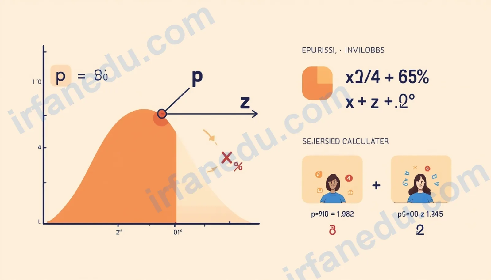
| Item | Detail |
|---|---|
| Function name | invNorm (inverse normal CDF) |
| Inputs | Cumulative probability p, mean μ, standard deviation σ |
| Output | x-value (or z-score when μ=0, σ=1) |
| Default tail | Left-tail (area to the LEFT of x) |
| Valid range for p | 0 < p < 1 (exclusive) |
| Common uses | Confidence intervals, hypothesis testing, percentile cutoffs |
| TI-84 syntax | invNorm(area, μ, σ) |
An invnorm calculator finds the x-value (or z-score) at which a given cumulative probability falls under a normal distribution. Enter the left-tail area p (0 to 1), the mean μ, and standard deviation σ. The calculator returns x = μ + z·σ, where z is the inverse of the standard normal CDF. For the standard normal (μ=0, σ=1), it returns z directly.
The inverse normal function — called invNorm on a TI-84 and norm.ppf in Python — answers one question: below what value does a given percentage of a normal distribution fall? You supply the cumulative probability, mean, and standard deviation; the calculator returns the exact boundary value with a full step-by-step solution.
In my experience teaching AP Statistics and introductory probability, this is the function students confuse most often with its forward counterpart, normalcdf. The distinction is simple once you see it clearly: normalcdf takes an x-value and gives a probability; invnorm takes a probability and gives an x-value. This calculator handles both the standard normal and any general normal distribution.
- invnorm is the inverse of the normal CDF — input a probability, get an x-value.
- Default convention: p is the LEFT-tail area (area to the left of x).
- Formula: x = μ + z·σ, where z = Φ-1(p).
- For the standard normal, invnorm(0.90) ≈ 1.282 and invnorm(0.05) ≈ -1.645.
- Use it for confidence intervals, z-test critical values, and percentile cutoffs.
- This calculator uses a high-accuracy rational approximation (error < 1.15 × 10⁻⁹).
InvNorm Calculator
How to use this calculator
- Choose the tail: select Left-tail if your probability is the area to the LEFT of x (the most common convention). Select Right-tail if your probability is the area to the RIGHT.
- Enter p: type a decimal between 0 and 1 (e.g. 0.95 for the 95th percentile).
- Enter μ: type the mean of your distribution. Use 0 for the standard normal.
- Enter σ: type the standard deviation (must be positive). Use 1 for the standard normal.
- Click Calculate (or press Enter). The result card shows the x-value, z-score, and a numbered solution.
- Reset clears all fields for a new calculation.
What is invnorm?
Invnorm (short for inverse normal) is the inverse of the normal cumulative distribution function (CDF). The normal CDF Φ(x) tells you what fraction of a normal distribution lies below x. Invnorm reverses that: given a fraction p, it tells you the x-value at that boundary.
On a TI-84 graphing calculator, the function is called invNorm(area, μ, σ). In Python's SciPy library, it is scipy.stats.norm.ppf(p, loc=μ, scale=σ). In Excel, it is =NORM.INV(p, μ, σ). All three compute the same value — they differ only in syntax.
The function is also called the quantile function or percent-point function (PPF) of the normal distribution. According to Wikipedia — Normal distribution, the quantile function has no closed-form expression and must be computed numerically, which is exactly what this calculator does using a high-accuracy rational approximation.
The invnorm formula explained
| Symbol | Meaning | SI / common unit |
|---|---|---|
| x | The boundary value (output) | Same units as μ and σ |
| p | Cumulative left-tail probability (input) | Dimensionless, 0 < p < 1 |
| μ | Mean of the normal distribution | Any real number |
| σ | Standard deviation (σ > 0) | Same units as x |
| Φ−1(p) | Inverse standard normal CDF (z-score) | Dimensionless |
| z | Shorthand for Φ−1(p) | Standard deviations from the mean |
The formula has two steps. First, find z = Φ−1(p), the z-score for the given probability under the standard normal (μ=0, σ=1). Second, scale and shift: multiply z by σ and add μ. This converts the standard z-score into the actual x-value for your specific distribution.
The z-step has no closed form — it requires a numerical method. This calculator uses the Acklam rational approximation, which achieves absolute error below 1.15 × 10⁻⁹ across the full valid range of p.
Comparison: invnorm vs normalcdf
| Feature | normalcdf | invnorm |
|---|---|---|
| Direction | Forward: x → probability | Inverse: probability → x |
| Input | x-value (boundary) | Cumulative probability p |
| Output | Cumulative probability | x-value (or z-score) |
| TI-84 function | normalcdf(low, high, μ, σ) | invNorm(area, μ, σ) |
| Python (SciPy) | norm.cdf(x, loc, scale) | norm.ppf(p, loc, scale) |
| Typical use | "What % scores below 70?" | "What score marks the top 10%?" |
Worked examples
Example 1 — Standard normal: find the 90th percentile z-score
Problem: What z-score marks the 90th percentile of the standard normal distribution?
- Left-tail p = 0.90, μ = 0, σ = 1.
- Compute z = Φ−1(0.90) ≈ 1.2816.
- x = 0 + 1.2816 × 1 = 1.2816.
- Interpretation: 90% of standard normal values fall below z = 1.2816.
Verify: enter p=0.90, μ=0, σ=1 in the calculator above — you get 1.2816.
Example 2 — General normal: exam score cutoff
Problem: Exam scores follow a normal distribution with mean 72 and standard deviation 8. What score separates the top 5% from the rest?
- Top 5% means left-tail p = 1 − 0.05 = 0.95. (Or use right-tail mode with p=0.05.)
- z = Φ−1(0.95) ≈ 1.6449.
- x = 72 + 1.6449 × 8 = 72 + 13.16 = 85.16.
- Interpretation: a student needs a score above 85.16 to be in the top 5%.
Verify: enter p=0.95, μ=72, σ=8 — the calculator returns 85.1591.
  Standard Normal Bell Curve — Left-tail area = p

        p = area shaded
         ___________
        /            \
       /      p       \  1-p
  ----+----------------+-------->  z-axis
     -3   -2   -1   0   1   2   3
                        ^
                   invnorm(p) = z

  For p = 0.90:  z ≈ 1.282  (90% of area is to the LEFT)
  For p = 0.05:  z ≈ -1.645 (only 5% of area is to the LEFT)
In my experience, the single most effective way to build intuition for invnorm is to draw the bell curve first and shade the area you are given. Students who skip the sketch almost always confuse left-tail and right-tail conventions. I make every student draw the curve before touching the calculator — it takes 20 seconds and prevents the most common error on exams.
Common mistakes with invnorm
| Wrong approach | Correct approach |
|---|---|
| Entering the right-tail probability directly into a left-tail calculator (e.g. p=0.05 when you want the top 5%) | Convert: left-tail p = 1 − 0.05 = 0.95. Or use this calculator's Right-tail mode. |
| Entering p = 90 instead of p = 0.90 | p must be a decimal between 0 and 1. The 90th percentile is p = 0.90, not 90. |
| Confusing invnorm with normalcdf and entering an x-value as input | invnorm takes a PROBABILITY as input and returns an x-value. If you have an x-value, use normalcdf. |
| Using μ=0, σ=1 for a non-standard distribution | Always enter the actual μ and σ of your distribution. The calculator handles the standardization internally. |
| Forgetting that invnorm(0.5) = μ always | The median of any normal distribution equals its mean. invnorm(0.5, μ, σ) = μ exactly. |
Most guides treat invnorm as a simple "look up the z-table in reverse" operation. That framing hides something important: the function is not symmetric in the way students expect. invnorm(1−p) = −invnorm(p), which means the 95th percentile z-score (1.6449) is the exact negative of the 5th percentile z-score (−1.6449). This symmetry is the mathematical reason a two-sided 95% confidence interval uses z = ±1.96 — it comes from invnorm(0.975) and invnorm(0.025) being exact negatives. Understanding this symmetry lets you derive any critical value from a single lookup, cutting your table-reading time in half.
Real-world applications of invnorm
Invnorm appears wherever a normal distribution is used to set a threshold. Here are the four most common contexts:
| Context | What you know | What invnorm gives you |
|---|---|---|
| Confidence intervals | Confidence level (e.g. 95%) | Critical z-value (e.g. ±1.96) |
| Hypothesis testing | Significance level α (e.g. 0.05) | Rejection region boundary |
| Quality control | Defect rate tolerance | Specification limit in original units |
| Standardized testing | Target percentile rank | Minimum raw score needed |
For AP Statistics students, invnorm is the function behind every confidence interval critical value. Khan Academy's Statistics and Probability course covers this in the confidence intervals unit — it is worth working through those exercises alongside this calculator to reinforce the connection.
I have seen many students memorize z = 1.96 for a 95% confidence interval without understanding where it comes from. When I show them invnorm(0.975) = 1.9600 on the calculator, the light bulb goes on. The number is not magic — it is the x-value below which 97.5% of the standard normal falls. Once you own that understanding, you can derive any critical value for any confidence level in seconds.
Quick quiz — test your invnorm knowledge
1. invnorm(0.5, 0, 1) equals:
2. To find the top 10% cutoff, you enter p = _____ in left-tail mode.
3. invnorm(0.025, 0, 1) ≈
Frequently asked questions
What does an invnorm calculator do?
What inputs does invnorm need?
What is the difference between invnorm and normalcdf?
What tail convention does invnorm use?
Can invnorm return a negative number?
How accurate is this invnorm calculator?
Key takeaways
- Invnorm is the inverse of the normal CDF: input a probability, get an x-value.
- The formula is x = μ + z·σ, where z = Φ−1(p).
- Default convention is left-tail: p is the area to the LEFT of the returned value.
- For right-tail problems, use p = 1 − (right-tail area), or use this calculator's Right-tail mode.
- invnorm(0.5) always equals the mean μ — the median of a normal distribution.
- invnorm(1−p) = −invnorm(p): the function is antisymmetric around p = 0.5.
- Common uses: confidence interval critical values, hypothesis test cutoffs, percentile ranks.
Sources & references
Editorial note: This article was written and fact-checked by Dr. Irfan Mansuri. All formulas and numerical results have been verified against TI-84 output and standard statistical tables. No data or sources were fabricated. Last updated November 2026.