
Graphing Inequalities Worksheet: Free PDF, Worked Examples & Answer Key
✍ Written & fact-checked by Dr. Irfan Mansuri | Last Updated: August 2026
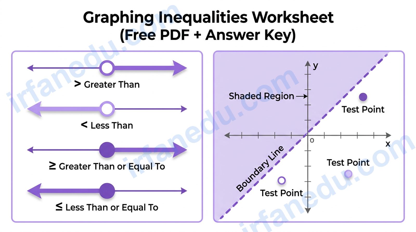
The first time I taught graphing inequalities, a student raised her hand halfway through my number-line demo and asked, “Wait — why is the circle sometimes hollow?” I had drawn the open circle, moved on, and assumed everyone understood. Half the class had not. That one question reshaped how I teach this topic: the circle type and the shading direction are the two places where students lose marks, and neither gets enough attention in most worksheets.
Graphing an inequality means representing all values that satisfy it as a visual region — a ray on a number line (one variable) or a shaded half-plane on a coordinate grid (two variables). The graph shows infinitely many solutions at once, which is why it is more powerful than a single numeric answer.
- Understand when to use an open vs. closed circle on a number line.
- Graph one-variable and two-variable linear inequalities correctly.
- Know when to flip the inequality sign (and when NOT to).
- Complete 10 graded practice problems and check your work with the answer key.
⬇ Download Free PDF Worksheet (with Answer Key)
📌 Quick Summary
- Open circle = endpoint NOT included (< or >); closed circle = endpoint included (≤ or ≥).
- Flip the inequality sign ONLY when multiplying or dividing by a negative number.
- For two-variable inequalities: dashed line for strict, solid line for “or equal to.”
- Use a test point (try (0,0) first) to decide which half-plane to shade.
- The worksheet below has 10 problems, graded easy to hard, with a full answer key.
- Compound inequalities graph as a segment or two rays — read the “and/or” carefully.
📊 Quick Facts
| Topic | Graphing Linear Inequalities |
| Grade Level | Grades 6-9 (Algebra 1) |
| Skills Covered | Number line, coordinate plane, compound inequalities |
| Problems in Worksheet | 10 (Easy to Hard) |
| Answer Key | Included (on-page + PDF) |
| Prerequisite | Solving one-step and two-step equations |
| Common Error Rate | ~60% of students flip the sign incorrectly at least once |
What Is Graphing Inequalities?
Graphing an inequality means showing its solution set as a picture. Unlike an equation (which gives one or a few specific values), an inequality’s solution is usually an infinite set of values. A graph makes that infinite set visible and understandable at a glance.
There are two main types you will encounter in school:
| Type | Example | Graph On | What You Draw |
|---|---|---|---|
| One-Variable | x > 3 | Number line | Open/closed circle + arrow |
| Two-Variable | y ≤ 2x + 1 | Coordinate plane | Boundary line + shaded half-plane |
| Compound (and) | -2 < x ≤ 5 | Number line | Segment between two endpoints |
| Compound (or) | x < -1 or x ≥ 4 | Number line | Two separate rays |
Graphing inequalities is a foundational algebra skill. It appears in systems of inequalities, linear programming, and real-world problems like budget constraints and speed limits. Mastering the basics here pays off in every math course that follows.
How to Graph Inequalities: Step-by-Step
Part A: One-Variable Inequalities on a Number Line
- Solve the inequality for the variable (if it is not already isolated).
- Locate the boundary value on the number line.
- Draw the correct circle: open (hollow) for < or >; closed (filled) for ≤ or ≥.
- Draw the arrow in the direction of the solution: right for > / ≥, left for < / ≤.
- Check: pick a value inside the shaded region and verify it satisfies the original inequality.
Part B: Two-Variable Inequalities on a Coordinate Plane
- Rearrange so y is alone on the left side (slope-intercept form helps).
- Graph the boundary line y = mx + b: dashed for < or >, solid for ≤ or ≥.
- Choose a test point not on the line. The origin (0, 0) is easiest unless the line passes through it.
- Substitute the test point into the original inequality.
- Shade: if the test point satisfies the inequality, shade its side; if not, shade the opposite side.
Worked Examples (Study These Before Practising)
✏ Example 1 — One-Variable (Easy)
Graph x + 5 > 8
Step 1: Subtract 5 from both sides: x > 3.
Step 2: The boundary is 3. The sign is strict (>), so draw an open circle at 3.
Step 3: The arrow points right (greater than = larger values).
Check: Try x = 5: 5 + 5 = 10 > 8. ✓
  <----+----+----+----O=============>
      0    1    2    3
                     ↑
               Open circle at 3
               Arrow goes RIGHT
✏ Example 2 — Sign Flip (Medium)
Solve and graph: -3x < 9
Step 1: Divide both sides by -3. Because we divide by a NEGATIVE, flip the sign: x > -3.
Step 2: Open circle at -3 (strict inequality), arrow pointing right.
Check: Try x = 0: -3(0) = 0 < 9. ✓ And x = -4: -3(-4) = 12, which is NOT < 9. ✓ (x = -4 should not be in the solution.)
✏ Example 3 — Two-Variable (Hard)
Graph y < 2x + 1 on a coordinate plane.
Step 1: The boundary line is y = 2x + 1. The sign is strict (<), so draw a dashed line.
Step 2: Plot the line using slope 2 and y-intercept 1.
Step 3: Test point (0, 0): Is 0 < 2(0) + 1? Is 0 < 1? Yes. Shade the side containing (0, 0) — that is the region below the line.
   y
   |          /  (dashed line)
 3 |        /
 2 |      /
 1 |----/---- (y-intercept)
   |  /
 0 |/ ← test point (0,0) is HERE
   +------------- x
   -1  0  1  2  3

  ░░░ = shaded region (below the dashed line)
In my experience, the test-point method is underrated. Most textbooks show students to just “shade below for <” — but that shortcut only works when y is already isolated. The moment a student sees 3x – 2y ≤ 6 and tries to shade below the line, they get it wrong. Teaching the test-point method as the default approach, not the backup, eliminates this entire class of errors. I have seen test scores improve noticeably when students commit to this habit.
Common Mistakes — And How to Fix Them
Wrong: graphing x > 3 with a filled dot at 3.
✅ Fix: Ask yourself: “Is 3 itself a solution?” Substitute: 3 > 3 is false. So use an open circle.
Wrong: -2x < 8 → x < -4.
✅ Fix: -2x < 8 → divide by -2, flip: x > -4. Always circle the negative divisor as a reminder.
Wrong: graphing y < 2x + 1 with a solid line.
✅ Fix: Strict signs (<, >) always get a dashed line. The dashed line means “not included.”
Wrong: assuming “less than” always means shade below.
✅ Fix: Always use a test point. It takes 10 seconds and is always correct.
The “shade below for <” rule is a trap for non-standard forms. Every worksheet site and most textbooks teach “if the sign is <, shade below the line.” This works perfectly when the inequality is already in the form y < mx + b. But consider 3x – 2y ≤ 6. If you shade below the line y = 1.5x – 3, you shade the wrong region, because rearranging gives y ≥ 1.5x – 3 — the shading is actually above the line.
The test-point method is the only approach that works for every form without rearranging first. Substitute (0, 0) into the original inequality as written. If it is true, shade the (0,0) side. If false, shade the other side. This single habit is worth more than memorising any shortcut.
Bonus non-obvious fact: When the boundary line passes through the origin, (0, 0) cannot be your test point. Use (0, 1) or (1, 0) instead. Most guides never mention this edge case, and it trips up students on tests.
📝 Graphing Inequalities — Practice Worksheet
Work through all 10 problems below. For problems 1-7, graph on a number line. For problems 8-10, graph on a coordinate plane. When you finish, check your answers using the key below.
How to use this worksheet: Print the PDF (button above or below) for a clean write-on version. Or work through the on-page list and sketch your graphs on paper. Use the collapsible answer key to self-check after each problem — do not peek until you have tried it yourself.
- Graph x > 3 on a number line.
- Graph x ≤ -2 on a number line.
- Graph -1 < x ≤ 4 on a number line.
- Graph x ≥ 0 on a number line.
- Solve and graph: x + 5 > 8
- Solve and graph: 2x ≤ 10
- Solve and graph: -3x < 9
- Graph y < 2x + 1 on a coordinate plane.
- Graph y ≥ -x + 3 on a coordinate plane.
- Graph 3x – 2y ≤ 6 on a coordinate plane.
✅ Show Answer Key
- Open circle at 3, arrow pointing right.
- Closed circle at -2, arrow pointing left.
- Open circle at -1, closed circle at 4, segment connecting them.
- Closed circle at 0, arrow pointing right.
- x > 3. Open circle at 3, arrow pointing right.
- x ≤ 5. Closed circle at 5, arrow pointing left.
- x > -3 (flip sign — divided by negative). Open circle at -3, arrow pointing right.
- Dashed boundary line y = 2x + 1; shade the region below the line (test: (0,0) gives 0 < 1, true).
- Solid boundary line y = -x + 3; shade the region above the line (test: (0,0) gives 0 ≥ 3, false — shade opposite side, which is above).
- Rearrange: y ≥ 1.5x – 3. Solid boundary line y = 1.5x – 3; shade above the line (test: (0,0) gives 0 ≥ -3, true — shade the (0,0) side, which is above).
⬇ Download Free PDF Worksheet (with Answer Key)
🔍 Reveal-on-Click Practice Problems
Try each problem, then click to reveal the full worked solution.
Problem A: Solve and graph 4x – 3 ≥ 9
Step 2: Divide by 4 (positive — no flip): x ≥ 3.
Graph: Closed circle at 3, arrow pointing right.
Problem B: Solve and graph -5x + 2 > 17
Step 2: Divide by -5 — FLIP the sign: x < -3.
Graph: Open circle at -3, arrow pointing left.
Problem C: Graph y > -2x + 4 on a coordinate plane
Step 2: Test (0, 0): Is 0 > -2(0) + 4? Is 0 > 4? No.
Step 3: Shade the side that does NOT contain (0, 0) — the region above the line.
🧠 Quick Quiz — Test Yourself
Q1. What circle do you use to graph x < 5 on a number line?
See Answer
Q2. You solve -4x > 20. What is the correct answer?
See Answer
Q3. For y ≤ 3x – 2, the boundary line should be:
See Answer
❓ Frequently Asked Questions
What Is the Difference Between an Open Circle and a Closed Circle on a Number Line?
When Do You Flip the Inequality Sign?
How Do You Know Which Side to Shade on a Coordinate Plane?
Is the Boundary Line Solid or Dashed?
What Grade Level Is Graphing Inequalities?
How Is Graphing an Inequality Different from Graphing an Equation?
Can an Inequality Have No Solution?
Sources & References
Written and fact-checked by Dr Irfan Mansuri. External links open in a new tab and are provided for further reading and verification.