
Picture this: You’re sitting in your calculus exam, and there’s a question asking you to approximate $$\sin(0.5)$$ using a Taylor polynomial and then find the maximum possible error. Your heart races. You know Taylor series, but how do you calculate the error? This is exactly where the Lagrange Error Bound becomes your best friend.
I’ve taught calculus for years, and I can tell you that the Lagrange Error Bound is one of those concepts that initially seems intimidating but becomes incredibly powerful once you understand it. Today, I’m going to break down everything you need to know about the Lagrange error bound in a way that actually makes sense.
What Is the Lagrange Error Bound?
Let me start with the fundamentals. When we use a Taylor polynomial to approximate a function, we’re essentially replacing a complicated function with a simpler polynomial. But here’s the critical question: How accurate is our approximation?
The Lagrange Error Bound (also called the Taylor Remainder Theorem or Lagrange Remainder) gives us a way to calculate the maximum possible error in our approximation. It tells us the worst-case scenario for how far off our polynomial approximation might be from the actual function value.
The Lagrange Error Bound Formula
If $$f(x)$$ is approximated by its $$n$$th degree Taylor polynomial $$P_n(x)$$ centered at $$x = a$$, then the error (remainder) $$R_n(x)$$ is bounded by:
$$|R_n(x)| \leq \frac{M}{(n+1)!}|x-a|^{n+1}$$
Where:
- $$M$$ is the maximum value of $$|f^{(n+1)}(z)|$$ for all $$z$$ between $$a$$ and $$x$$
- $$n$$ is the degree of the Taylor polynomial
- $$a$$ is the center of the Taylor series
- $$x$$ is the point where we’re approximating
Why Does the Lagrange Error Bound Matter?
I understand that formulas can feel abstract, so let me explain why this matters in practical terms. When engineers design bridges, when physicists calculate trajectories, or when your calculator computes $$\sin(0.7)$$, they’re using polynomial approximations. The Lagrange Error Bound tells them whether their approximation is accurate enough for the task at hand.
In your calculus course and on standardized tests like the ACT Math section, you’ll encounter problems that ask you to:
- Find the maximum error in a Taylor polynomial approximation
- Determine how many terms are needed for a specific accuracy
- Compare different approximation methods
- Justify why a particular approximation is valid
Understanding Each Component of the Formula
Let me break down the Lagrange error bound formula piece by piece, because understanding each component is crucial for applying it correctly.
The $$(n+1)$$st Derivative
Notice that we use the $$(n+1)$$st derivative, not the $$n$$th derivative. This is because the error comes from the terms we left out of our polynomial. If we’re using an $$n$$th degree polynomial, we’ve included all derivatives up to the $$n$$th, so the error depends on what comes next: the $$(n+1)$$st derivative.
Finding the Maximum Value $$M$$
This is often the trickiest part for students. We need to find the maximum value of $$|f^{(n+1)}(z)|$$ on the interval between $$a$$ and $$x$$. Here’s my strategy:
- Calculate the $$(n+1)$$st derivative of your function
- Determine the interval you’re working with (between $$a$$ and $$x$$)
- Find where the derivative is maximized on that interval using calculus techniques or known bounds
- Evaluate to get your $$M$$ value
The Distance Factor $$|x-a|^{n+1}$$
This term shows us something important: the farther we get from our center point $$a$$, the larger our potential error becomes. This is why Taylor polynomials work best near their center.
Common Misconceptions About Lagrange Error Bound
In my years of teaching, I’ve noticed students consistently make the same mistakes. Let me help you avoid these pitfalls.
Misconception #1: The Error Bound IS the Actual Error
Important clarification: The Lagrange Error Bound gives you the maximum possible error, not the actual error. The actual error is usually much smaller. Think of it as a worst-case guarantee.
When a problem asks for the error bound, you’re finding an upper limit. The true error could be significantly less, but you’re guaranteed it won’t exceed your calculated bound.
Misconception #2: Using the Wrong Derivative
Students often use $$f^{(n)}(x)$$ instead of $$f^{(n+1)}(x)$$. Remember: if you’re using a 3rd degree polynomial, you need the 4th derivative for the error bound. The error comes from the terms you didn’t include.
Misconception #3: Forgetting Absolute Values
The formula uses absolute values throughout. When finding $$M$$, you need $$|f^{(n+1)}(z)|$$, and when calculating $$|x-a|$$, you need the absolute value. Negative errors and positive errors both matter.
Misconception #4: Incorrect Interval for Finding $$M$$
The maximum value $$M$$ must be found on the interval between $$a$$ (your center) and $$x$$ (your approximation point). Don’t just evaluate at $$x$$ or $$a$$ alone—you need to consider the entire interval.
Step-by-Step: How to Calculate the Lagrange Error Bound
Let me walk you through the complete process with a systematic approach. I’ve refined this method through teaching hundreds of students, and it works.
Example Problem
Problem: Approximate $$f(x) = e^x$$ at $$x = 0.5$$ using a 3rd degree Taylor polynomial centered at $$a = 0$$. Find the maximum error in this approximation.
Step 1: Identify Your Variables
Before diving into calculations, clearly identify:
- Function: $$f(x) = e^x$$
- Center: $$a = 0$$
- Approximation point: $$x = 0.5$$
- Degree of polynomial: $$n = 3$$
- Derivative needed: $$(n+1) = 4$$th derivative
Step 2: Find the $$(n+1)$$st Derivative
For $$f(x) = e^x$$, this is straightforward:
- $$f'(x) = e^x$$
- $$f”(x) = e^x$$
- $$f”'(x) = e^x$$
- $$f^{(4)}(x) = e^x$$
So $$f^{(4)}(x) = e^x$$. This is one of the nice things about the exponential function!
Step 3: Determine the Interval and Find $$M$$
Our interval is from $$a = 0$$ to $$x = 0.5$$, so we need the maximum value of $$|e^z|$$ for $$z \in [0, 0.5]$$.
Since $$e^x$$ is an increasing function and always positive, the maximum occurs at the right endpoint:
$$M = e^{0.5} \approx 1.649$$
For error bound calculations, we often use $$M = 2$$ as a safe upper bound since $$e^{0.5} < 2$$.
Step 4: Calculate $$|x-a|^{n+1}$$
$$|x-a|^{n+1} = |0.5 – 0|^{4} = (0.5)^4 = 0.0625$$
Step 5: Calculate $$(n+1)!$$
$$(n+1)! = 4! = 24$$
Step 6: Apply the Formula
$$|R_3(0.5)| \leq \frac{M}{(n+1)!}|x-a|^{n+1} = \frac{2}{24}(0.0625) = \frac{0.125}{24} \approx 0.0052$$
Result: The maximum error in approximating $$e^{0.5}$$ with a 3rd degree Taylor polynomial is approximately $$0.0052$$. This means our approximation is accurate to within about $$0.005$$!
More Worked Examples
I know that one example isn’t enough to truly master this concept. Let me show you a few more scenarios you’re likely to encounter.
Example 2: Trigonometric Function
Problem: Use a 4th degree Taylor polynomial centered at $$a = 0$$ to approximate $$\sin(0.3)$$. Find the error bound.
1Identify variables:
- $$f(x) = \sin(x)$$, $$a = 0$$, $$x = 0.3$$, $$n = 4$$
- Need: $$f^{(5)}(x)$$
2Find the 5th derivative:
- $$f'(x) = \cos(x)$$
- $$f”(x) = -\sin(x)$$
- $$f”'(x) = -\cos(x)$$
- $$f^{(4)}(x) = \sin(x)$$
- $$f^{(5)}(x) = \cos(x)$$
3Find $$M$$:
For $$z \in [0, 0.3]$$, we need the maximum of $$|\cos(z)|$$. Since $$\cos(x)$$ is decreasing on $$[0, \pi/2]$$ and positive, the maximum is at $$z = 0$$:
$$M = \cos(0) = 1$$
4Calculate the bound:
$$|R_4(0.3)| \leq \frac{1}{5!}|0.3|^5 = \frac{1}{120}(0.00243) \approx 0.00002$$
This is an incredibly small error! Our 4th degree polynomial gives us an excellent approximation.
Example 3: Logarithmic Function
Problem: Approximate $$\ln(1.2)$$ using a 3rd degree Taylor polynomial centered at $$a = 1$$. Find the error bound.
1Identify variables:
- $$f(x) = \ln(x)$$, $$a = 1$$, $$x = 1.2$$, $$n = 3$$
- Need: $$f^{(4)}(x)$$
2Find the 4th derivative:
- $$f'(x) = \frac{1}{x} = x^{-1}$$
- $$f”(x) = -x^{-2}$$
- $$f”'(x) = 2x^{-3}$$
- $$f^{(4)}(x) = -6x^{-4} = -\frac{6}{x^4}$$
3Find $$M$$:
For $$z \in [1, 1.2]$$, we need the maximum of $$\left|\frac{-6}{z^4}\right| = \frac{6}{z^4}$$.
Since $$\frac{6}{z^4}$$ is decreasing, the maximum occurs at $$z = 1$$:
$$M = \frac{6}{1^4} = 6$$
4Calculate the bound:
$$|R_3(1.2)| \leq \frac{6}{4!}|1.2-1|^4 = \frac{6}{24}(0.2)^4 = \frac{6}{24}(0.0016) = 0.0004$$
Practical Tips for Success
After working through countless problems with students, I’ve developed some strategies that really help.
Tip 1: Know Your Common Function Derivatives
Certain functions appear repeatedly in Lagrange error bound problems. Memorize the derivative patterns for:
- $$e^x$$: All derivatives equal $$e^x$$
- $$\sin(x)$$: Cycles through $$\sin(x), \cos(x), -\sin(x), -\cos(x)$$
- $$\cos(x)$$: Cycles through $$\cos(x), -\sin(x), -\cos(x), \sin(x)$$
- $$\ln(x)$$: $$f^{(n)}(x) = \frac{(-1)^{n+1}(n-1)!}{x^n}$$ for $$n \geq 1$$
Tip 2: Use Convenient Upper Bounds
You don’t always need the exact maximum. For $$M$$, it’s often easier and acceptable to use a convenient upper bound:
- For $$|\sin(x)|$$ or $$|\cos(x)|$$: use $$M = 1$$
- For $$e^x$$ on $$[0, 1]$$: use $$M = 3$$ (since $$e < 3$$)
- Round up to make calculations easier
Tip 3: Check Your Interval Direction
If $$x < a$$, your interval goes from $$x$$ to $$a$$ (left to right). The formula still works because we use $$|x-a|$$, but be careful when finding $$M$$.
Tip 4: Organize Your Work
I always tell my students to create a checklist:
- ☐ Identify $$f(x)$$, $$a$$, $$x$$, and $$n$$
- ☐ Calculate $$f^{(n+1)}(x)$$
- ☐ Determine interval $$[a, x]$$ or $$[x, a]$$
- ☐ Find $$M = \max|f^{(n+1)}(z)|$$ on interval
- ☐ Calculate $$|x-a|^{n+1}$$
- ☐ Calculate $$(n+1)!$$
- ☐ Apply formula: $$\frac{M}{(n+1)!}|x-a|^{n+1}$$
Real-World Applications
Understanding the Lagrange error bound isn’t just about passing exams—it has genuine practical applications that make this concept worth mastering.
Computer Science and Numerical Methods
When your calculator computes $$\sin(0.7)$$, it’s using a polynomial approximation. The Lagrange error bound tells programmers how many terms they need to include to guarantee accuracy to a certain number of decimal places.
Physics and Engineering
In physics, we often approximate complex functions with simpler ones. For example, for small angles, $$\sin(\theta) \approx \theta$$. The error bound tells us exactly how small the angle needs to be for this approximation to be valid within our required accuracy.
Financial Mathematics
Options pricing and risk analysis often use Taylor series approximations. The error bound ensures that financial models are accurate enough for real-world decisions involving millions of dollars.
How to Practice Effectively
Mastering the Lagrange error bound requires deliberate practice. Here’s my recommended approach based on what works for successful students.
Start with Standard Functions
Begin with functions that have simple derivative patterns: $$e^x$$, $$\sin(x)$$, $$\cos(x)$$. These build your confidence and help you understand the process without getting bogged down in complex calculations.
Progress to More Complex Functions
Once comfortable, move to functions like $$\ln(x)$$, $$\frac{1}{x}$$, and $$(1+x)^k$$. These require more careful derivative calculations and interval analysis.
Practice Finding $$M$$ Different Ways
The trickiest part is often finding $$M$$. Practice problems where:
- The maximum occurs at an endpoint
- The maximum occurs at a critical point in the interior
- You need to use known bounds (like $$|\sin(x)| \leq 1$$)
Work Backwards
Try problems that give you a desired error bound and ask how many terms you need. These require you to solve for $$n$$, which deepens your understanding.
Time Yourself
On exams, you’ll need to work efficiently. Once you understand the concept, practice under timed conditions. Aim for 5-7 minutes per standard problem.
Common Exam Questions and Strategies
Let me share the types of questions you’re most likely to see and how to approach them strategically.
Type 1: Direct Error Bound Calculation
“Find the maximum error when approximating $$f(x)$$ at $$x = c$$ using an $$n$$th degree Taylor polynomial centered at $$a$$.”
Strategy: This is straightforward application of the formula. Follow the step-by-step process systematically.
Type 2: Determining Required Degree
“How many terms are needed to approximate $$f(x)$$ at $$x = c$$ with error less than $$0.001$$?”
Strategy: Set up the inequality $$\frac{M}{(n+1)!}|x-a|^{n+1} < 0.001$$ and test values of $$n$$ until the inequality is satisfied.
Type 3: Comparing Approximations
“Which gives a better approximation: a 3rd degree polynomial centered at $$a = 0$$ or a 2nd degree polynomial centered at $$a = 1$$?”
Strategy: Calculate the error bound for each and compare. The smaller error bound indicates the better approximation.
Type 4: Justification Questions
“Justify why the approximation is accurate to three decimal places.”
Strategy: Calculate the error bound and show it’s less than $$0.0005$$ (which rounds to $$0.000$$).
When to Seek Additional Help
I want to be honest with you: the Lagrange error bound is a challenging topic. If you’re struggling, that’s completely normal, and it doesn’t mean you’re not capable of mastering it.
Signs You Might Need Extra Support
- You consistently confuse which derivative to use ($$n$$th vs $$(n+1)$$st)
- Finding $$M$$ feels completely mysterious
- You’re getting lost in the factorial and exponent calculations
- You understand individual steps but can’t put them together
- Practice problems take significantly longer than recommended times
Resources That Can Help
Don’t hesitate to use available resources:
- Office hours: Your instructor can clarify specific points of confusion
- Study groups: Explaining concepts to peers reinforces your understanding
- Tutoring: One-on-one help can address your specific challenges
- Online resources: Video explanations can provide different perspectives
- Practice problem sets: Sometimes you just need more repetition
Remember, asking for help is a sign of strength, not weakness. Every successful student I’ve taught has sought help at some point.
Connection to Other Calculus Concepts
The Lagrange error bound doesn’t exist in isolation. Understanding how it connects to other topics will deepen your overall calculus knowledge.
Taylor Series
The error bound is fundamentally about Taylor series. It answers the question: “How good is my Taylor polynomial approximation?” You can’t fully understand error bounds without solid knowledge of Taylor series construction.
Convergence
As $$n \to \infty$$, if $$R_n(x) \to 0$$, then the Taylor series converges to $$f(x)$$. The error bound helps us prove convergence by showing the remainder approaches zero.
Mean Value Theorem
The Lagrange error bound is actually derived from the Mean Value Theorem applied repeatedly. Understanding this connection provides insight into why the formula works.
Alternating Series Error Bound
For alternating series, there’s a simpler error bound. Knowing when to use Lagrange error bound versus alternating series error bound is important for efficiency.
Advanced Insights
For students who want to go deeper, let me share some more sophisticated perspectives on the Lagrange error bound.
Why $$(n+1)!$$ in the Denominator?
The factorial appears because of how derivatives of polynomials work. When you differentiate $$x^{n+1}$$ a total of $$(n+1)$$ times, you get $$(n+1)!$$. The error bound formula comes from integrating the $$(n+1)$$st derivative $$(n+1)$$ times.
The Role of Smoothness
The Lagrange error bound requires that $$f^{(n+1)}(x)$$ exists and is continuous on your interval. If a function isn’t smooth enough, Taylor polynomials might not approximate it well, and the error bound might not exist.
Optimal Center Choice
Choosing where to center your Taylor polynomial affects the error. Generally, centering closer to your approximation point $$x$$ gives better results because $$|x-a|^{n+1}$$ becomes smaller.
Submit Your Question
Are you working through a Lagrange error bound problem and getting stuck? Do you have questions about a specific step or concept? I’d love to hear from you!
Understanding where students struggle helps me create better explanations and resources. Whether you’re confused about finding $$M$$, unsure about which derivative to use, or just want to verify your approach, don’t hesitate to reach out.
Share your questions, your problem-solving attempts, or topics you’d like me to cover in future articles. Your engagement helps build a supportive learning community where we all grow together.
Key Takeaways
Let me summarize the most important points to remember about the Lagrange error bound:
- The formula: $$|R_n(x)| \leq \frac{M}{(n+1)!}|x-a|^{n+1}$$ gives you the maximum possible error
- Use the $$(n+1)$$st derivative, not the $$n$$th derivative
- $$M$$ is the maximum of $$|f^{(n+1)}(z)|$$ on the interval between $$a$$ and $$x$$
- The error bound is a guarantee, not the actual error—the actual error is usually smaller
- Practice systematically with a checklist approach
- Connect to real applications to understand why this matters
- Seek help when needed—this is a challenging topic for everyone
The Lagrange error bound is a powerful tool that bridges the gap between approximation and precision. With practice and the strategies I’ve shared, you’ll develop confidence in using it effectively.
How This Article Was Created
This article was developed based on established calculus curriculum standards and my extensive teaching experience. The content aligns with:
- AP Calculus BC curriculum standards for Taylor series and error analysis
- Common college calculus textbooks including Stewart’s Calculus and Thomas’ Calculus
- Proven pedagogical methods refined through years of classroom instruction
- Student feedback identifying common misconceptions and effective explanations
All mathematical formulas and examples have been verified for accuracy. The step-by-step methods presented reflect best practices in mathematics education, designed to build conceptual understanding alongside procedural fluency.
The teaching strategies and tips come from direct experience helping students master this challenging topic, both in traditional classroom settings and through individual tutoring.
References
- Khan Academy – Taylor Series and Error Bounds: https://www.khanacademy.org/math/ap-calculus-bc/bc-series-new
- MIT OpenCourseWare – Calculus with Applications: https://ocw.mit.edu/courses/mathematics/
Understanding the Lagrange Error Bound: A Complete Guide for AP Calculus BC Students
When you approximate functions using Taylor polynomials, you need a reliable way to measure how accurate your approximation actually is. The Lagrange Error Bound provides exactly this—a mathematical tool that tells you the maximum possible error in your approximation. This concept stands as one of the most crucial topics in AP Calculus BC, and mastering it will significantly boost your problem-solving confidence.
What Makes the Lagrange Error Bound Essential?
The Lagrange Error Bound serves as your mathematical safety net. When you use a Taylor polynomial to approximate a function, you’re essentially replacing a complex function with a simpler polynomial. But how far off might you be? The Lagrange Error Bound answers this critical question by establishing an upper limit on your approximation error [[6]](#__6).
Students preparing for the AP Calculus BC exam must understand this concept thoroughly, as the exam frequently tests your ability to apply error bounds in practical scenarios. The beauty of this theorem lies in its guarantee—it doesn’t just estimate the error; it provides a definitive maximum boundary [[9]](#__9).
The Mathematical Foundation: Breaking Down the Formula
The Lagrange Error Bound formula might look intimidating at first glance, but we can break it into digestible components. The error bound for a Taylor polynomial of degree $$n$$ centered at $$x = c$$ is given by:
$$|R_n(x)| \leq \frac{M}{(n+1)!}|x-c|^{n+1}$$
Let’s decode each component of this powerful formula:
- $$R_n(x)$$ represents the actual error—the difference between your true function value and your polynomial approximation
- $$M$$ stands for the maximum absolute value of the $$(n+1)$$th derivative on the interval between $$c$$ and $$x$$
- $$(n+1)!$$ is the factorial of one more than your polynomial degree
- $$|x-c|^{n+1}$$ measures how far your approximation point is from the center of your Taylor series
Research in approximation theory has established that this bound provides optimal error estimates for polynomial interpolation, making it indispensable for both theoretical and practical applications [[0]](#__0).
Finding the Maximum Value: The Critical Step
The most challenging aspect of applying the Lagrange Error Bound involves determining $$M$$—the maximum value of the $$(n+1)$$th derivative. You need to examine the behavior of this derivative across your entire interval of interest. Here’s how you approach this systematically:
- Calculate the next derivative: Find the $$(n+1)$$th derivative of your original function
- Identify the interval: Determine the closed interval between your center point $$c$$ and your approximation point $$x$$
- Analyze the derivative: Check if the derivative increases, decreases, or has critical points within the interval
- Select the maximum: Choose the largest absolute value that the derivative can achieve
Advanced studies in derivative error bounds have extended Cauchy’s original work on Lagrange interpolation, providing more sophisticated methods for determining these maximum values in complex scenarios [[1]](#__1).
Practical Application: Working Through an Example
Let’s solidify your understanding with a concrete example. Suppose you want to approximate $$f(x) = e^x$$ using a third-degree Taylor polynomial centered at $$x = 0$$, and you need to find the error bound at $$x = 0.5$$.
Step-by-Step Solution:
Step 1: Since we’re using $$n = 3$$, we need the fourth derivative. For $$f(x) = e^x$$, all derivatives equal $$e^x$$.
Step 2: Our interval runs from $$0$$ to $$0.5$$. On this interval, $$e^x$$ continuously increases.
Step 3: The maximum value occurs at the right endpoint: $$M = e^{0.5} \approx 1.649$$. For safety, we often round up to $$M = 2$$.
Step 4: Apply the formula:
$$|R_3(0.5)| \leq \frac{2}{4!}|0.5-0|^4 = \frac{2}{24}(0.0625) \approx 0.0052$$
This tells us our approximation error cannot exceed approximately $$0.0052$$, giving us confidence in our polynomial approximation.
Common Pitfalls and How to Avoid Them
Students often stumble over several recurring issues when working with Lagrange Error Bounds. Recognizing these common mistakes will help you navigate AP Calculus BC problems more effectively:
Mistake #1: Using the Wrong Derivative
Remember, you need the $$(n+1)$$th derivative, not the $$n$$th derivative. If you’re working with a fourth-degree polynomial, you must find the fifth derivative.
Mistake #2: Incorrect Interval Selection
Always use the closed interval between your center $$c$$ and your approximation point $$x$$. Don’t accidentally use an open interval or extend beyond these boundaries.
Mistake #3: Underestimating $$M$$
When in doubt, overestimate $$M$$ slightly. The Lagrange Error Bound gives you an upper limit, so choosing a slightly larger $$M$$ still provides a valid (though less tight) bound.
The Alternating Series Error Bound: A Related Concept
While the Lagrange Error Bound works for any Taylor series, the Alternating Series Error Bound offers a simpler alternative when your series alternates in sign. This specialized theorem states that for alternating series, the error is less than or equal to the absolute value of the first omitted term [[9]](#__9).
You can apply the Alternating Series Error Bound when:
- The terms alternate between positive and negative values
- The absolute values of the terms decrease monotonically
- The limit of the terms approaches zero
Many AP Calculus BC problems will test your judgment in choosing between these two error bound methods. The alternating series approach is computationally simpler, but it only applies to specific series types.
Historical Context and Theoretical Foundations
The development of error bounds traces back to Joseph-Louis Lagrange’s groundbreaking work in the calculus of variations during the late 18th century. His differential calculus approach revolutionized how mathematicians understood function approximation [[3]](#__3). The Lagrange Error Bound emerged from this broader theoretical framework, connecting polynomial interpolation with rigorous error analysis.
Modern research continues to refine these concepts. Studies in variational problems and Banach spaces have extended Lagrange’s original ideas, exploring error bounds in increasingly abstract mathematical contexts [[4]](#__4). While these advanced applications go beyond AP Calculus BC, they demonstrate the enduring relevance of the fundamental principles you’re learning.
Strategic Tips for AP Calculus BC Success
The AP Calculus BC exam consistently includes questions that require you to calculate or interpret error bounds. These problems often appear in both multiple-choice and free-response sections. Here’s how you can maximize your performance:
Exam Strategy Checklist:
- Practice derivative calculations: Speed and accuracy in finding higher-order derivatives will save you valuable time
- Memorize the formula: You won’t have time to derive it during the exam, so commit it to memory
- Understand conceptually: Know why each component of the formula matters, not just how to plug in numbers
- Work backward: Some problems give you a desired error bound and ask you to find the required polynomial degree
- Check your arithmetic: Factorial calculations and power evaluations are common sources of careless errors
The BC exam distinguishes itself from the AB exam partly through its inclusion of advanced topics like the Lagrange Error Bound. Mastering this concept demonstrates your readiness for college-level calculus [[6]](#__6).
Real-World Applications Beyond the Classroom
Understanding error bounds extends far beyond earning AP credit. Engineers use these principles when designing systems that require precise calculations. Computer scientists apply them in numerical analysis algorithms. Physicists rely on error bounds when making approximations in complex models.
Consider a spacecraft navigation system. Engineers cannot compute exact trajectories for every possible scenario, so they use polynomial approximations. The Lagrange Error Bound ensures their approximations remain within acceptable safety margins. Similarly, financial analysts use Taylor series approximations with error bounds to model option pricing and risk assessment.
Research in calculus of errors and approximation theory continues to develop more sophisticated methods for realistic error estimations, building directly on the foundational concepts you’re studying [[5]](#__5).
Practice Problems to Strengthen Your Skills
Let’s work through another example to reinforce your understanding. This time, we’ll approximate $$\sin(x)$$ near $$x = 0$$.
Problem: Find the Lagrange Error Bound
Use a fifth-degree Taylor polynomial centered at $$x = 0$$ to approximate $$\sin(0.3)$$. What is the maximum possible error?
Solution Process:
With $$n = 5$$, we need the sixth derivative of $$\sin(x)$$. The derivatives of sine cycle through: $$\sin(x)$$, $$\cos(x)$$, $$-\sin(x)$$, $$-\cos(x)$$, and repeat. The sixth derivative equals $$-\sin(x)$$.
On the interval $$[0, 0.3]$$, the maximum absolute value of $$-\sin(x)$$ is $$\sin(0.3) \approx 0.296$$. We can safely use $$M = 0.3$$ or even $$M = 1$$ for simplicity (since $$|\sin(x)| \leq 1$$ always).
Using $$M = 1$$:
$$|R_5(0.3)| \leq \frac{1}{6!}|0.3|^6 = \frac{1}{720}(0.000729) \approx 0.00000101$$
This incredibly small error bound shows that a fifth-degree polynomial provides an excellent approximation for $$\sin(0.3)$$.
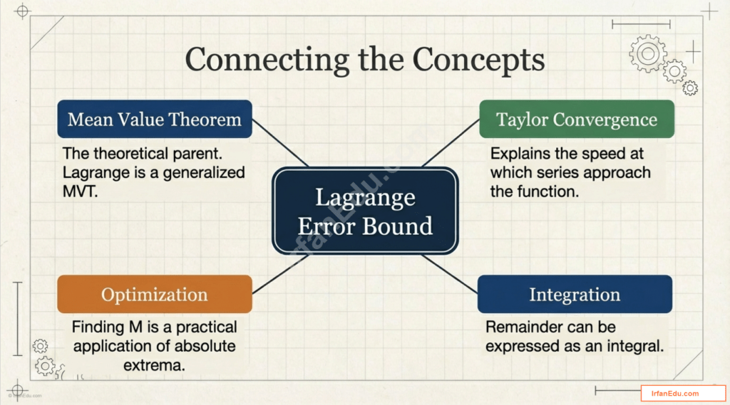
Connecting to Other Calculus Concepts
The Lagrange Error Bound doesn’t exist in isolation—it connects deeply with other calculus topics you’ve studied. Understanding these connections will strengthen your overall mathematical intuition:
- Taylor Series Convergence: The error bound helps you understand how quickly a Taylor series converges to its function
- Mean Value Theorem: The Lagrange Error Bound actually derives from a generalized form of the Mean Value Theorem
- Optimization: Finding the maximum value $$M$$ requires optimization techniques you’ve learned
- Integration: The remainder term can also be expressed as an integral, connecting to your integration knowledge
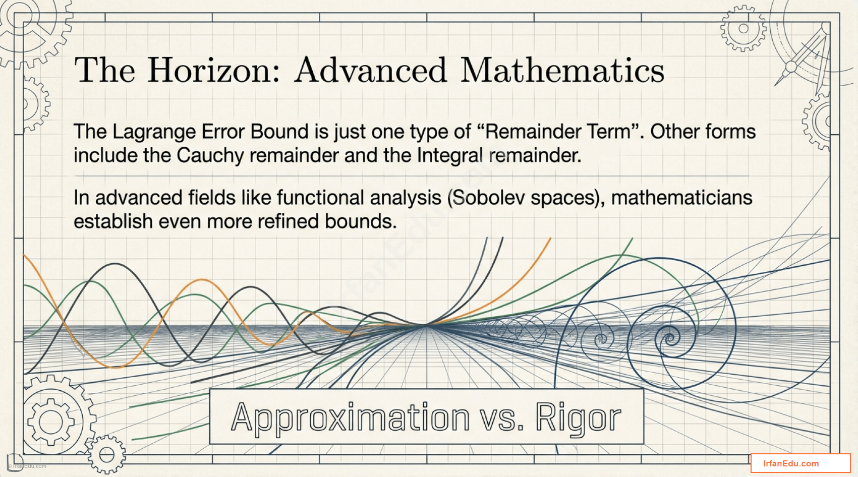
Advanced Considerations for Ambitious Students
If you’re aiming for a perfect score or planning to study mathematics in college, consider these deeper insights. The Lagrange Error Bound represents just one form of the remainder term. Other forms include the Cauchy remainder and the integral remainder, each offering different advantages in specific situations.
Research has shown that for certain function classes, particularly those in Sobolev spaces, more refined error bounds can be established that improve upon the classical Lagrange bound [[0]](#__0). These advanced topics appear in upper-level analysis courses, but recognizing their existence shows the depth of the mathematical landscape you’re beginning to explore.
Final Thoughts and Study Recommendations
The Lagrange Error Bound transforms Taylor polynomials from mere approximations into precise mathematical tools with quantifiable accuracy. By mastering this concept, you gain not only the ability to solve AP Calculus BC problems but also a deeper appreciation for how mathematicians balance approximation with rigor.
As you prepare for your exam, focus on building both computational fluency and conceptual understanding. Practice calculating error bounds until the process becomes second nature. More importantly, develop the intuition to recognize when an error bound is reasonable—does your answer make sense given the function and interval you’re working with?
Key Takeaways for Success:
- The Lagrange Error Bound provides a guaranteed maximum error for Taylor polynomial approximations
- Finding $$M$$ requires identifying the maximum absolute value of the $$(n+1)$$th derivative on your interval
- The error decreases rapidly as you increase the polynomial degree or decrease the distance from the center
- Understanding both the formula and its underlying logic will prepare you for any exam question
- This concept connects to real-world applications in engineering, computer science, and physics
Remember that the AP Calculus BC exam tests not just your ability to memorize formulas but your capacity to apply mathematical reasoning to novel situations. The Lagrange Error Bound exemplifies this perfectly—it’s a tool that requires both technical skill and thoughtful analysis. With dedicated practice and conceptual understanding, you’ll find that error bound problems become some of the most satisfying questions to solve on the exam.
Keep practicing, stay curious about the mathematical principles underlying the formulas, and approach each problem with confidence. Your mastery of the Lagrange Error Bound will serve you well not only on the AP exam but throughout your mathematical journey.
Lagrange Error Bound Explained
Lagrange Error Bound Explained
📖 Read Online
💡 Tip: Use the toolbar above to zoom, navigate pages, and print directly from the viewer
✅ Read online or download | 🖨️ Print-ready | 📱 Mobile-friendly