
Heart model in math: the equation, graph, and how it works 💜
If I could teach you one thing about this topic, it would be this: the heart model in math is not just a fun trick for Valentine’s Day — it is a genuine gateway into some of the most important ideas in high school and college math. I have used it in classrooms to introduce implicit equations, polar coordinates, and parametric curves, and every time, students who were bored by abstract algebra suddenly leaned forward.
The moment you type (x²+y²−1)³ = x²y³ into Desmos and a perfect heart appears on the screen, something clicks. Math stops being a list of rules and starts being a language that can describe anything — even something as human as a heart shape.
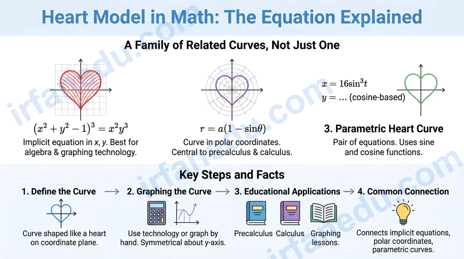
The heart model in math refers to any curve whose graph resembles a heart shape. The most famous is the algebraic heart curve defined by the implicit equation (x² + y² − 1)³ = x²y³. A second major form is the polar cardioid r = a(1 − sinθ). A third is the parametric Valentine curve using sine and cosine. All three are real mathematical objects studied in algebra, precalculus, and calculus.
- 🎯 You will understand what the heart model equation actually means — not just what it looks like.
- 📐 You will be able to graph the heart curve by hand and with a calculator.
- 🔄 You will know the difference between the algebraic, polar, and parametric versions.
- 🚫 You will avoid the three most common mistakes students make with this topic.
- 💡 You will see why this curve matters beyond aesthetics — it connects to real math concepts you are already studying.
Core idea: The heart model is not one equation — it is a family of related curves. Knowing which version you are working with (algebraic, polar, or parametric) is the first step to understanding it correctly.
⚡ In Short
- 💜 The heart model is any math curve that looks like a heart shape.
- 📝 The algebraic heart curve equation is (x² + y² − 1)³ = x²y³.
- 🌀 The polar cardioid r = a(1 − sinθ) is the most common heart in polar graphing.
- 📊 The parametric heart uses x = 16sin³t and a cosine-based y formula.
- 🔍 All three curves are symmetric about the y-axis (or the polar axis).
- 🎓 These curves appear in precalculus, calculus, and graphing technology lessons worldwide.
What is the heart model in math?
The heart model in math is any curve defined by a mathematical equation whose graph on a coordinate plane forms a recognizable heart shape. It is not a single equation — it is a family of related curves, each arising from a different branch of mathematics.
Three main versions exist and each one teaches something different:
- The algebraic heart curve — an implicit equation in x and y, best for algebra and graphing technology lessons.
- The polar cardioid — a curve in polar coordinates, central to precalculus and calculus.
- The parametric heart curve — a pair of equations using a parameter t, used in calculus and computer graphics.
The word “cardioid” itself comes from the Greek kardia, meaning heart. Mathematicians have studied cardioids since at least the 17th century, and the algebraic heart curve became famous in the internet age when it started circulating as a “math love equation.”
In my experience teaching this, students almost always search for “the heart equation” expecting one answer. The biggest service I can do is show them there are three distinct versions — and that each one connects to a different chapter of their math textbook. Once they see that, the heart model stops being a novelty and starts being a revision tool.
The algebraic heart curve equation
The algebraic heart curve is defined by the implicit equation (x² + y² − 1)³ = x²y³. This single equation, when graphed, produces a smooth heart shape with a cusp at the bottom and a dip at the top.
Let me break down what each part of the equation does:
- (x² + y² − 1) — this expression equals zero on the unit circle. Raising it to the third power stretches the curve away from that circle.
- x²y³ — this term controls the asymmetry between the top and bottom of the curve. The y³ term (odd power) allows the bottom to form a pointed cusp while the top stays rounded.
- The cube on the left — the exponent 3 is what creates the characteristic dip at the top. Without it, you get a very different shape.
📌 Worked example: verifying a point on the heart curve
Does the point (1, 0) lie on the curve (x² + y² − 1)³ = x²y³?
Left side: (1² + 0² − 1)³ = (1 + 0 − 1)³ = (0)³ = 0
Right side: 1² × 0³ = 1 × 0 = 0
Left = Right ✓ — yes, (1, 0) is on the curve. By symmetry, (−1, 0) is also on the curve.
📌 Worked example: checking the top dip point
Does (0, 1) lie on the curve?
Left side: (0 + 1 − 1)³ = 0³ = 0
Right side: 0² × 1³ = 0
Left = Right ✓ — yes, (0, 1) is on the curve. This is the top center of the heart (the dip point).
The curve is symmetric about the y-axis. You can verify this algebraically: replace x with −x in the equation. Since x appears only as x², the equation is unchanged. This means the left half mirrors the right half perfectly.
How to graph the heart curve step by step
Graphing the algebraic heart curve is straightforward with a graphing tool, and achievable by hand with a few key points. Here is the full process.
Using Desmos (recommended for students)
- Go to desmos.com/calculator.
- Click on the expression field and type:
(x^2+y^2-1)^3 = x^2*y^3 - Press Enter. The heart shape appears immediately in purple (or your chosen color).
- Zoom in to see the cusp at the bottom and the dip at the top clearly.
- Use the “wrench” settings to adjust the window if needed (try x: −2 to 2, y: −2 to 1.5).
🖼 ASCII art: heart curve key features
        y
        |
   1.0  +    *       *
        |  *   *   *   *
   0.5  + *       *       *
        |*                 *
   0.0  +---*-----------*------- x
        | *               *
  -0.5  |  *             *
        |    *         *
  -1.0  |      *     *
        |        * *
  -1.25 +         * (cusp)
        |
        +--+--+--+--+--+--+--
          -1.5  0   1.5

  Key points:
  • Top dip:      (0,  1.0)
  • Widest:       (±1, 0.0)
  • Bottom cusp:  (0, ~-1.25)
  • Symmetry:     y-axis
Graphing by hand (approximate sketch)
- Plot the verified points: (0, 1), (1, 0), (−1, 0), and (0, −1.25).
- Draw two rounded lobes from (−1, 0) and (1, 0) up to (0, 1), with a slight inward dip at (0, 1).
- From (±1, 0), curve downward and inward to meet at the cusp (0, −1.25).
- The result is a smooth heart shape. The bottom point is sharp (a cusp), not rounded.
✅ Pro tip: the cusp is not a corner
Many students draw the bottom of the heart as a sharp angular corner. In reality, the algebraic heart curve has a cusp — a point where the curve comes to a smooth but pointed tip. The tangent line is vertical there, not angled. When sketching by hand, make the bottom tip narrow and smooth, not jagged.
The polar cardioid: another heart model
The polar cardioid is the heart model you encounter in precalculus and calculus when studying polar coordinates. Its equation is r = a(1 − sinθ), where a is a positive constant that controls the size of the curve.
A cardioid is defined geometrically as the path traced by a point on the rim of a circle that rolls around another circle of equal radius. This mechanical definition is beautiful — it means the heart shape is not arbitrary, but arises naturally from circular motion.
📌 Worked example: plotting the cardioid r = 1 − sinθ
For the cardioid r = 1 − sinθ, calculate r at key angles:
- θ = 0°: r = 1 − sin(0) = 1 − 0 = 1
- θ = 90°: r = 1 − sin(90°) = 1 − 1 = 0 (the cusp — at the origin)
- θ = 180°: r = 1 − sin(180°) = 1 − 0 = 1
- θ = 270°: r = 1 − sin(270°) = 1 − (−1) = 2 (the widest point, at the bottom)
Plot these (r, θ) pairs in polar coordinates and connect them smoothly. The cusp appears at the top (θ = 90°) and the widest point is at the bottom (θ = 270°). This gives a heart shape pointing downward — rotate it 180° mentally to match the classic orientation.
To get a heart pointing upward (the classic orientation), use r = a(1 + sinθ) instead. The plus sign flips the curve vertically.
✅ Orientation tip: sin vs cos
Use r = a(1 ± sinθ) for a cardioid oriented vertically (cusp at top or bottom). Use r = a(1 ± cosθ) for a cardioid oriented horizontally (cusp pointing left or right). This is a detail many textbooks gloss over that costs students marks on graphing questions.
The parametric heart curve
The parametric heart curve is the most visually precise version and the one used most often in computer graphics and art. It expresses x and y separately as functions of a parameter t, where t runs from 0 to 2π.
The most popular parametric heart equations are:
- x(t) = 16 sin³(t)
- y(t) = 13 cos(t) − 5 cos(2t) − 2 cos(3t) − cos(4t)
These equations produce a smooth, symmetric, anatomically-inspired heart shape. The x equation uses sin³(t) — a cubed sine — which creates the rounded lobes. The y equation is a sum of cosine harmonics that shapes the top dip and the bottom cusp simultaneously.
📌 Worked example: parametric heart at t = 0 and t = π/2
At t = 0:
- x = 16 sin³(0) = 16 × 0 = 0
- y = 13(1) − 5(1) − 2(1) − 1 = 13 − 5 − 2 − 1 = 5
- Point: (0, 5) — the top center of the heart.
At t = π/2:
- x = 16 sin³(π/2) = 16 × 1³ = 16
- y = 13 cos(π/2) − 5 cos(π) − 2 cos(3π/2) − cos(2π) = 0 − (−5) − 0 − 1 = 4
- Point: (16, 4) — the rightmost lobe of the heart.
In Desmos, enter the parametric form by clicking the “+” button and selecting “parametric.” Then type the two equations with t as the parameter. The result is a large, smooth heart — the same shape you see in math memes and Valentine’s Day cards across the internet.
Comparing the three heart models
Each heart model has a different equation form, coordinate system, and use case. Here is a direct comparison to help you choose the right one for your purpose.
| Feature | Algebraic heart curve | Polar cardioid | Parametric heart |
|---|---|---|---|
| Equation | (x²+y²−1)³ = x²y³ | r = a(1 − sinθ) | x=16sin³t, y=13cost−5cos2t−2cos3t−cos4t |
| Coordinate system | Cartesian (x, y) | Polar (r, θ) | Parametric (t) |
| Equation type | Implicit | Explicit polar | Explicit parametric |
| Symmetry | y-axis | Polar axis (vertical) | y-axis |
| Cusp location | Bottom (0, ~−1.25) | Top (θ = 90°, r = 0) | Bottom (0, −13) |
| Best for | Algebra, graphing tech | Polar coordinates unit | Calculus, computer graphics |
| Graph in Desmos | (x^2+y^2-1)^3=x^2*y^3 | r=1-sin(theta) | Parametric mode, t: 0 to 2π |
Common mistakes students make with the heart model
In my experience, students make the same three errors repeatedly when working with heart curves. Here they are — and how to fix each one.
❌ Mistake 1: confusing the cardioid with the heart curve
Wrong thinking: “The cardioid and the algebraic heart curve are the same equation.”
Correct: They are different equations in different coordinate systems. The cardioid r = a(1 − sinθ) is a polar curve. The algebraic heart (x²+y²−1)³ = x²y³ is a Cartesian implicit curve. They look similar but are mathematically distinct objects. On an exam, using the wrong one will cost you marks.
❌ Mistake 2: thinking the heart curve is a function
Wrong thinking: “I can write y = f(x) for the heart curve.”
Correct: The algebraic heart curve is an implicit equation — it cannot be written as a single function y = f(x) because for most x values, there are multiple y values. This is why you cannot graph it by entering “y =” in a standard graphing calculator — you need an implicit graphing tool like Desmos.
❌ Mistake 3: wrong orientation for the polar cardioid
Wrong thinking: “r = 1 − sinθ gives a heart pointing upward.”
Correct: r = 1 − sinθ gives a heart with the cusp at the top (θ = 90°) and the wide part at the bottom — so it points downward. To get the classic upward-pointing heart, use r = 1 + sinθ. Many students get this backwards on polar graphing tests.
What I find genuinely exciting about the heart model is that it sits at the intersection of three different coordinate systems — Cartesian, polar, and parametric. Most students encounter these systems as separate, disconnected chapters. The heart curve is one of the few topics that lets you say: “Here is the same idea expressed three different ways.” That cross-system thinking is exactly what standardized tests and university math courses reward. I always use the heart model as a capstone activity at the end of the graphing unit for this reason.
The algebraic heart curve is not the “true” heart equation — it was popularized by a viral internet post, not by mathematicians. The equation (x²+y²−1)³ = x²y³ was circulated widely online as a romantic math fact, but it is not a named curve in classical mathematics the way the cardioid is. The cardioid has a 350-year history, appears in antenna design, microphone polar patterns, and the Mandelbrot set’s main bulb boundary. The algebraic heart curve, by contrast, is a modern construction chosen specifically because it looks good on a screen.
This matters for students because: if your teacher asks about “the heart curve in polar coordinates,” they almost certainly mean the cardioid — not the viral internet equation. Knowing the difference prevents a very common exam error. The parametric version is also far more useful in calculus and physics than the algebraic one, yet it gets almost no attention in popular math content.
Where the heart model appears in real math and science
The heart model is not just decorative. Each version connects to real applications in mathematics, engineering, and physics.
The cardioid in acoustics and antenna design
Cardioid microphones are named after the cardioid curve because their pickup pattern — the region from which they capture sound — is shaped like a cardioid. Engineers describe this pattern using the polar equation r = a(1 + cosθ). The same shape appears in directional antennas used in radio and telecommunications.
[IMAGE: Cardioid microphone pickup pattern diagram | ALT: cardioid polar pattern diagram showing heart-shaped sound pickup zone for microphone]
The cardioid in the Mandelbrot set
The main bulb of the Mandelbrot set — the iconic fractal shape — is bounded by a cardioid. The boundary of the main cardioid of the Mandelbrot set is defined by the equation c = μ/2 − μ²/4, where μ = e^(iθ). This is a direct connection between the heart model and one of the most famous objects in modern mathematics.
Parametric curves in computer graphics
The parametric heart curve is used in graphic design software, animation, and game development to draw smooth heart shapes programmatically. Any time you see a heart shape in a digital interface — an app icon, a loading animation, a social media “like” button — the underlying shape is often defined by a parametric or Bézier curve closely related to the parametric heart equations.
Implicit curves in algebraic geometry
The algebraic heart curve is an example of an algebraic curve — a curve defined by a polynomial equation in x and y. Algebraic geometry, a major branch of university mathematics, studies these curves systematically. The heart curve is a degree-6 algebraic curve (the highest power in the equation is 6, from x² × y³ × … when expanded), which places it in a rich mathematical family.
Practice problems: test your understanding 🧪
Work through these problems on your own, then click to reveal the solution.
Problem 1: Does the point (0, −1) lie on the algebraic heart curve (x²+y²−1)³ = x²y³?
Solution:
Left side: (0² + (−1)² − 1)³ = (0 + 1 − 1)³ = 0³ = 0
Right side: 0² × (−1)³ = 0 × (−1) = 0
Left = Right ✓ — yes, (0, −1) is on the curve. It sits on the lower part of the heart, above the cusp.
Problem 2: For the cardioid r = 2(1 − sinθ), find r when θ = 270°.
Solution:
sin(270°) = −1
r = 2(1 − (−1)) = 2(2) = 4
This is the maximum r value — the widest point of the cardioid, located at the bottom of the curve (pointing downward from the origin).
Problem 3: For the parametric heart, find the point (x, y) when t = π.
Solution:
x = 16 sin³(π) = 16 × 0³ = 0
y = 13 cos(π) − 5 cos(2π) − 2 cos(3π) − cos(4π)
= 13(−1) − 5(1) − 2(−1) − 1
= −13 − 5 + 2 − 1 = −17
Point: (0, −17) — the bottom cusp of the parametric heart.
Problem 4: Is the algebraic heart curve a function? Explain why or why not.
Solution:
No. A function requires exactly one y value for each x value. The heart curve has two y values for most x values between −1 and 1 (one on the upper half, one on the lower half). This fails the vertical line test. The curve is an implicit relation, not a function. This is why it cannot be entered as “y =” in a standard graphing calculator.
Problem 5: Write the polar cardioid equation for a heart that is widest at the right side (cusp pointing left).
Solution:
Use the cosine form: r = a(1 + cosθ)
At θ = 0°: r = a(1 + 1) = 2a (widest, pointing right)
At θ = 180°: r = a(1 + (−1)) = 0 (cusp, pointing left)
So r = a(1 + cosθ) gives a cardioid with the cusp on the left and the wide part on the right.
Frequently asked questions about the heart model in math
What is the heart model in math?
The heart model in math is a curve whose graph on a coordinate plane resembles a heart shape. The most famous version is the algebraic heart curve defined by (x² + y² − 1)³ = x²y³. A second common form is the polar cardioid r = a(1 − sinθ). A third is the