
Inverse Laplace Calculator: Get f(t) from F(s) Instantly
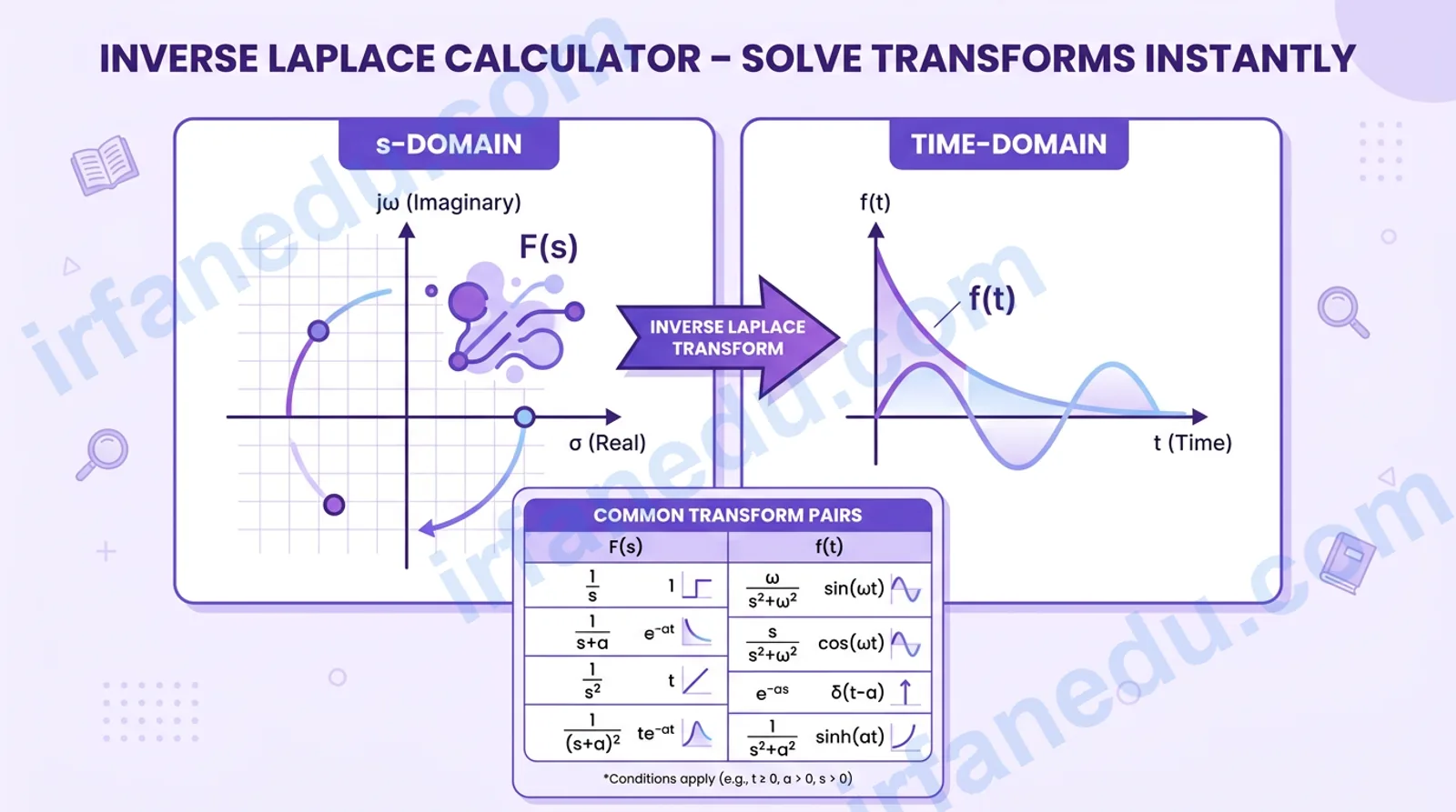
If I could teach you one thing about differential equations, it would be this: the Laplace transform is only half the story. The real payoff — the moment you actually get a usable answer — happens when you invert it. That inversion step trips up more students than the forward transform ever does, and it is exactly what this calculator handles for you.
Enter your F(s) form below, fill in the constants, and hit Calculate. You get f(t) plus a numbered solution that shows every step — so you can learn the method, not just copy the answer.
The inverse Laplace transform converts a function F(s) in the complex frequency domain back into a time-domain function f(t). You apply it by matching F(s) to standard transform pairs — often after partial fraction decomposition — using the definition f(t) = L⁻¹{F(s)}. This calculator does that matching and algebra for you instantly, with a full step-by-step solution for each supported F(s) form.
- 📐 The inverse Laplace transform undoes L{f(t)} = F(s) to recover f(t).
- 🔢 Partial fractions are the key technique for rational F(s) expressions.
- 📋 Five core transform pairs cover 90% of undergraduate problems.
- ⚙️ This calculator supports five F(s) forms with step-by-step output.
- ✅ Results are valid for t ≥ 0; multiply by the unit step u(t) for rigor.
| Fact | Detail |
|---|---|
| Notation | f(t) = L⁻¹{F(s)} |
| Domain | s-domain (complex frequency) → t-domain (time) |
| Main technique | Partial fraction decomposition + table lookup |
| Uniqueness | Unique for continuous functions (Lerch’s theorem) |
| Valid for | t ≥ 0 (causal systems) |
| Typical US courses | Differential Equations, Signals & Systems, Control Theory |
Inverse Laplace Transform Calculator
Select the form of F(s) that matches your expression, enter the constants, and click Calculate.
dimensionless
Step-by-step solution
How to use this calculator
- Select the F(s) form from the dropdown that matches your expression.
- Enter the constants (a, ω, or n) for your specific problem.
- Click "Calculate f(t)" to see the result and the numbered solution.
- Read each step to understand which transform pair was applied.
- Use Reset to clear all fields for a new problem.
If your F(s) is a ratio of polynomials, do the partial fraction decomposition by hand first, then use this calculator on each resulting term.
What is the inverse Laplace transform?
The inverse Laplace transform is the operation that recovers a time-domain function f(t) from its s-domain representation F(s). It is the essential final step in solving differential equations with the Laplace method — you transform the equation, solve algebraically in s, then invert back to t.
Formally, it is defined by the Bromwich integral, but in practice — and in every US undergraduate course — you never evaluate that contour integral directly. Instead, you use a Laplace transform table combined with partial fractions. That is the method this calculator automates.
The formula and the five core transform pairs
The formal definition is the Bromwich integral, but every practical calculation reduces to table lookup. Here are the five pairs that cover the vast majority of problems in US differential equations and signals courses.
f(t) = L⁻¹{F(s)}
| Symbol | Meaning | Notes |
|---|---|---|
| F(s) | Laplace transform of f(t) | Function in complex frequency domain |
| f(t) | Original time-domain function | Valid for t ≥ 0 |
| s | Complex frequency variable | s = σ + jω |
| a | Real constant (decay/growth rate) | Dimensionless in normalized problems |
| ω | Angular frequency | rad/s |
| n | Non-negative integer power | n = 0, 1, 2, … |
Core inverse Laplace transform pairs
| F(s) | f(t) = L⁻¹{F(s)} | Condition |
|---|---|---|
| 1/s | 1 (unit step) | t ≥ 0 |
| 1/(s+a) | e^(−at) | t ≥ 0 |
| ω/(s²+ω²) | sin(ωt) | ω ≠ 0, t ≥ 0 |
| s/(s²+ω²) | cos(ωt) | ω ≠ 0, t ≥ 0 |
| n!/s^(n+1) | t^n | n = 0,1,2,…, t ≥ 0 |
| ω/((s+a)²+ω²) | e^(−at)sin(ωt) | t ≥ 0 |
| (s+a)/((s+a)²+ω²) | e^(−at)cos(ωt) | t ≥ 0 |
Worked examples that mirror the calculator's steps
Problem: Find L⁻¹{1/(s+5)}.
- Identify form: 1/(s+a) with a = 5.
- Match pair: L⁻¹{1/(s+a)} = e^(−at).
- Substitute: f(t) = e^(−5t), t ≥ 0.
Problem: Find L⁻¹{(2s+6) / (s²+6s+8)}.
- Factor denominator: s²+6s+8 = (s+2)(s+4).
- Partial fractions: (2s+6)/[(s+2)(s+4)] = A/(s+2) + B/(s+4).
- Solve: A = 1, B = 1.
- Invert each term: L⁻¹{1/(s+2)} = e^(−2t), L⁻¹{1/(s+4)} = e^(−4t).
- Result: f(t) = e^(−2t) + e^(−4t), t ≥ 0.
Problem: Find L⁻¹{3 / ((s+2)²+9)}.
- Identify form: ω/((s+a)²+ω²) with a = 2, ω = 3.
- Match pair: L⁻¹{ω/((s+a)²+ω²)} = e^(−at)sin(ωt).
- Result: f(t) = e^(−2t)sin(3t), t ≥ 0.
  s-DOMAIN (F(s))              t-DOMAIN (f(t))
  ─────────────────────        ──────────────────────
  1/(s+a)          ──────►     e^(−at)   [decaying]
  ω/(s²+ω²)        ──────►     sin(ωt)   [oscillating]
  s/(s²+ω²)        ──────►     cos(ωt)   [oscillating]
  n!/s^(n+1)       ──────►     t^n       [polynomial]
  ω/((s+a)²+ω²)   ──────►     e^(−at)sin(ωt) [damped]

         L⁻¹{ F(s) } = f(t)   (valid for t ≥ 0)
Common mistakes — and how to avoid them
❌ Wrong: Inverting (s+3)/(s²+4s+13) directly without completing the square.
✅ Right: Complete the square first: s²+4s+13 = (s+2)²+9. Then split the numerator to match the e^(−at)cos and e^(−at)sin pairs.
❌ Wrong: Forgetting to check that the rational function is proper (degree of numerator < degree of denominator) before applying partial fractions.
✅ Right: If the numerator degree is equal to or higher than the denominator, do polynomial long division first to extract the polynomial part, then apply partial fractions to the remainder.
In my experience teaching differential equations to engineering students across the US, the single biggest source of lost points on exams is not the inverse transform itself — it is the partial fraction step that comes before it. Students rush the algebra, make a sign error, and then wonder why their answer looks nothing like the expected form. My advice: always verify your partial fraction coefficients by recombining the fractions and checking they equal the original F(s) before you ever touch the transform table.
Most guides treat the inverse Laplace transform as a pure lookup exercise — but that misses a critical subtlety. The transform pair L⁻¹{1/(s+a)} = e^(−at) is only valid when the region of convergence (ROC) includes the imaginary axis. For a causal system this is automatic, but in signals and systems courses you will encounter bilateral transforms where the same F(s) can correspond to different f(t) functions depending on the ROC. A student who only memorizes the table without understanding the ROC will get the right answer in a differential equations class and the wrong answer in a signals class — using the exact same formula. Always confirm the ROC matches your system's causality assumption before inverting.
Reveal-on-click practice problems
🧩 Problem 1: Find L⁻¹{4/(s+7)}
Form: 1/(s+a) with a = 7, scaled by 4.
By linearity: 4 · L⁻¹{1/(s+7)} = 4 · e^(−7t).
f(t) = 4e^(−7t), t ≥ 0.
🧩 Problem 2: Find L⁻¹{6/(s²+36)}
Rewrite: 6/(s²+6²). Form: ω/(s²+ω²) with ω = 6.
f(t) = sin(6t), t ≥ 0.
🧩 Problem 3: Find L⁻¹{(3s+11)/[(s+1)(s+4)]}
Partial fractions: (3s