
Regression Calculator: Find Your Line of Best Fit Instantly
You have a table of numbers and a question: what does the trend predict? Whether you are a high-school student running a science-fair experiment, a college student in an intro stats course, or a small-business owner eyeing sales data, linear regression gives you a precise, defensible answer. This calculator does the heavy lifting — enter your data pairs, hit Calculate, and you get the equation, R², and a prediction in under two minutes.
In my experience teaching statistics across high school and undergraduate courses, the single biggest time-waster students face is hand-computing the least-squares formulas. This tool eliminates that so you can focus on interpreting the result — which is the skill that actually matters on exams and in real life.
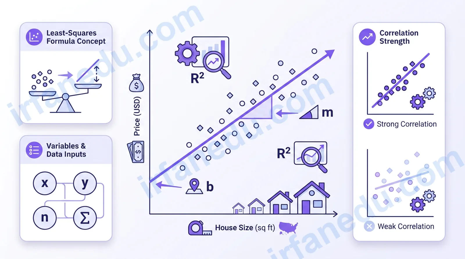
A regression calculator finds the best-fit straight line through a set of data points using the least-squares method. It outputs the slope (m), y-intercept (b), correlation coefficient (r), and R² value. Enter your x and y data pairs, click Calculate, and the tool instantly gives you the equation ŷ = mx + b plus a predicted y for any x you choose.
📌 Quick Summary
- 📐 Regression finds the line that minimizes total squared error across all data points.
- 📊 The output equation is ŷ = mx + b — slope m and intercept b are computed for you.
- 🔢 R² (0 to 1) tells you how much of the y-variation your line actually explains.
- 🎯 Use the Predict x field to forecast any y value from your fitted model.
- ⚠️ Correlation is not causation — a high R² does not prove x causes y.
- 🧮 Calculator
- How to Use
- What Is Regression?
- The Formula
- Worked Examples
- Common Mistakes
- Quiz
- FAQ
- Key Takeaways
Linear Regression Calculator
Enter data pairs → get slope, intercept, R², and a prediction
Enter at least 3 (x, y) pairs. Add rows as needed.
| # | x value | y value |
|---|---|---|
| 1 | ||
| 2 | ||
| 3 | ||
| 4 | ||
| 5 |
optional
📋 Step-by-Step Solution
Least-Squares Linear Regression fits the line ŷ = mx + b that minimizes the sum of squared vertical distances from each data point to the line.
| Symbol | Meaning | Unit |
|---|---|---|
| n | Number of data pairs | — |
| x, y | Independent and dependent variables | Any |
| Σ | Sum over all n data points | — |
| m | Slope (rise over run) | units of y per unit of x |
| b | y-intercept (value of ŷ when x = 0) | units of y |
| r | Pearson correlation coefficient (−1 to +1) | dimensionless |
| R² | Coefficient of determination (0 to 1) | dimensionless |
| ŷ | Predicted y value | units of y |
How to Use This Regression Calculator
- Enter your data pairs. Type each x value and its matching y value in the table rows. Leave blank rows empty — the calculator skips them.
- Add more rows by clicking + Add Row if you have more than five data points (up to 20 pairs).
- Enter a Predict x value (optional) if you want to forecast a specific y.
- Click “Calculate Regression.” The result card shows the equation, r, R², and your prediction.
- Check the step-by-step solution to see every intermediate sum — great for verifying homework or exam work.
What Is Linear Regression?
Linear regression is a statistical method that models the relationship between two variables by fitting a straight line to observed data. The line is chosen to minimize the sum of the squared vertical distances between each data point and the line — a criterion called least squares.
The result is the equation ŷ = mx + b, where m is the slope and b is the y-intercept. Once you have that equation, you can plug in any x value to predict the corresponding y — which is why regression is the backbone of forecasting in science, economics, and engineering.
The Regression Formula Explained
The least-squares formulas look intimidating at first, but each piece has a clear job. Here is a plain-English breakdown:
| Term | Formula | What It Measures |
|---|---|---|
| Slope (m) | (n·Σxy − Σx·Σy) / (n·Σx² − (Σx)²) | How much y changes for each 1-unit increase in x |
| Intercept (b) | (Σy − m·Σx) / n | The predicted y when x = 0 |
| Pearson r | Numerator of m / √(Var_x · Var_y) | Direction and strength of linear relationship (−1 to +1) |
| R² | r² | Proportion of y-variance explained by x (0 to 1) |
A key insight: the slope m is literally the covariance of x and y divided by the variance of x. That is why a larger spread in x gives you a more precise slope estimate — more x-variation means more information.
Worked Examples
Example 1 — Study Hours vs. Test Score
A US high-school teacher records five students’ weekly study hours (x) and their exam scores (y):
| Student | Study Hours (x) | Score (y) |
|---|---|---|
| 1 | 2 | 55 |
| 2 | 4 | 65 |
| 3 | 6 | 75 |
| 4 | 8 | 82 |
| 5 | 10 | 90 |
Step 1 — Sums: n = 5, Σx = 30, Σy = 367, Σxy = 2,330, Σx² = 220, Σy² = 27,219
Step 2 — Slope: m = (5×2330 − 30×367) / (5×220 − 30²) = (11650 − 11010) / (1100 − 900) = 640 / 200 = 3.2
Step 3 — Intercept: b = (367 − 3.2×30) / 5 = (367 − 96) / 5 = 271 / 5 = 54.2
Equation: ŷ = 3.2x + 54.2 — each extra study hour predicts 3.2 more points.
Predict 7 hours: ŷ = 3.2(7) + 54.2 = 22.4 + 54.2 = 76.6
r ≈ 0.996, R² ≈ 0.992 — study hours explain 99.2% of the score variation in this sample.
Score (y)
 90 |                              ●
 82 |                         ●
 75 |                    ●
 65 |          ●
 55 |    ●
    +----+----+----+----+----+----→ Hours (x)
    0    2    4    6    8   10
         ŷ = 3.2x + 54.2  (R²=0.992)
Example 2 — House Size vs. Sale Price (US)
A real-estate student pulls five recent sales from a Midwestern city: sizes in square feet (x) and prices in thousands of dollars (y).
Data: (1,000, 180), (1,400, 220), (1,800, 265), (2,200, 310), (2,600, 355)
Running this through the calculator gives: ŷ = 0.1x + 80, r = 0.9998, R² = 0.9996. A 2,000 sq ft home predicts $280,000 — very close to the observed $287,500 midpoint of the data.
R² does not tell you if your model is correct — it only tells you how well a straight line fits your