
Graphing radical functions: the complete step-by-step guide
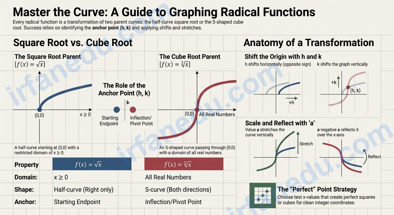
Graphing radical functions means plotting curves built from square roots or cube roots. The key steps are: identify the parent function, locate the anchor point, determine the domain, apply transformations in order, and plot a handful of test points. Every radical graph is just a shifted, stretched, or flipped version of one of two parent curves.
Think about the last time you watched a skateboarder roll up a half-pipe. The curve they follow — fast at the bottom, slowing as they rise — is almost exactly the shape of a square root function. The graph does not shoot straight up like a line; it curves and flattens. That visual intuition is the key to understanding radical graphs before you ever touch an equation.
In my experience teaching algebra, students who struggle with radical functions are almost always trying to memorize the graph shape instead of understanding why it curves. Once you see the analogy, the shape becomes obvious — and the transformations fall into place naturally.
- 🎯 Understand why radical graphs curve and flatten
- 🎯 Identify the two parent radical functions and their key features
- 🎯 Apply transformations (shifts, stretches, reflections) correctly
- 🎯 Find domain and range without a calculator
- 🎯 Avoid the three most common graphing errors
📌 Key takeaway: Every radical function you will ever graph is a transformation of either f(x) = √x or f(x) = ∛x. Master those two shapes and you have mastered the entire topic.
Graphing radical functions means plotting curves like f(x) = √x or f(x) = ∛x by identifying the parent function, finding the domain (x ≥ 0 for square root; all reals for cube root), applying transformations in order, and plotting key anchor points. The anchor point — where the graph starts or pivots — shifts with every horizontal and vertical translation.
📌 Quick Summary
- 📐 Two parent functions: f(x) = √x (half-curve) and f(x) = ∛x (S-curve).
- 🔢 Square root domain: x ≥ anchor value. Cube root domain: all real numbers.
- 📍 Anchor point = set the radicand to zero, solve for x, add vertical shift k.
- ↕ Vertical stretch ‘a’ multiplies y-values; negative ‘a’ flips the graph over x-axis.
- ⚠ Horizontal shifts go opposite to the sign inside the radical.
- 🧮 Always plot the anchor + at least two test points before drawing the curve.
The ramp analogy: why radical graphs look the way they do
Imagine filling a square swimming pool with water. As you add water, the depth increases — but the width of the water surface grows much more slowly. That relationship between area and side length is exactly √x. The more area you add, the less the side length grows per unit. That is why the graph curves and flattens: each extra unit of x produces a smaller and smaller increase in y.
Now formalize that intuition. The function f(x) = √x asks: “What number, squared, gives me x?” As x grows from 0 to 1, y jumps from 0 to 1 — a full unit. But as x grows from 100 to 101, y only moves from 10 to about 10.05. The same one-unit increase in x produces almost nothing in y. That is sublinear growth, and it is the defining visual feature of every square root graph.
🏊 Real-world anchor: The relationship between the area of a square and its side length is f(side) = √(area). A 4 m² pool has a 2 m side. A 9 m² pool has a 3 m side. A 100 m² pool has a 10 m side. Notice how the side length grows slower and slower — that is your radical graph in action.
The cube root function f(x) = ∛x is different. It is defined for all real numbers (including negatives), and its graph is S-shaped — it passes through the origin, rises to the right, and falls to the left. Think of it as the “balanced” radical: symmetric about the origin, never trapped on one side of the y-axis.
The two parent radical functions
A parent radical function is the simplest version of a radical equation — no shifts, no stretches, no reflections. Every transformed radical graph is built from one of these two foundations.
Parent function 1: f(x) = √x (square root)
- Domain: x ≥ 0 (you cannot take the square root of a negative number in the real number system)
- Range: y ≥ 0
- Starting point: (0, 0)
- Shape: Curves upward and to the right, flattening as x increases
- Key points: (0, 0), (1, 1), (4, 2), (9, 3), (16, 4)
Parent function 2: f(x) = ∛x (cube root)
- Domain: All real numbers (−∞, ∞)
- Range: All real numbers (−∞, ∞)
- Pivot point: (0, 0)
- Shape: S-shaped curve passing through the origin; odd symmetry (rotational symmetry about the origin)
- Key points: (−8, −2), (−1, −1), (0, 0), (1, 1), (8, 2)
  y
  4 |          * (16,4)         ← f(x)=√x
    |
  3 |       * (9,3)
    |
  2 |    * (4,2)                * (8,2) ← f(x)=∛x
    |
  1 | * (1,1)               * (1,1)
    |
  0 +--*--+--+--+--+--+--+--+--+--→ x
    |  0  1  2  3  4  5  6  7  8
 -1 |                       * (-1,-1)
    |
 -2 |                   * (-8,-2)
    |
  Key:  *=√x curve points   *=∛x curve points
  √x starts at (0,0) and curves right.
  ∛x passes through origin, extends both directions.
Quick facts at a glance
| Property | f(x) = √x | f(x) = ∛x |
|---|---|---|
| Domain | x ≥ 0 | All real numbers |
| Range | y ≥ 0 | All real numbers |
| Anchor / pivot point | (0, 0) | (0, 0) |
| Graph shape | Half-curve (right side only) | S-curve (both sides) |
| Symmetry | None | Odd (origin symmetry) |
| Negative x allowed? | No | Yes |
| Passes through origin? | Yes | Yes |
| Index of radical | 2 (even) | 3 (odd) |
How to find domain and range
The domain of a radical function is the set of x-values that produce real outputs. For square root functions, the expression under the radical must be greater than or equal to zero.
Finding the domain of a square root function
Set the radicand (expression inside the radical) ≥ 0 and solve for x.
📝 Example: Find the domain of f(x) = √(2x − 6).
Set 2x − 6 ≥ 0 → 2x ≥ 6 → x ≥ 3.
Domain: [3, ∞) — the graph starts at x = 3 and extends right.
Finding the range
For f(x) = a√(x − h) + k:
- If a > 0: range is y ≥ k (graph opens upward from anchor)
- If a < 0: range is y ≤ k (graph opens downward from anchor)
For cube root functions, the domain and range are always all real numbers — no restrictions needed.
Transformations: shifts, stretches, and reflections
Every radical function can be written in the general form f(x) = a√(x − h) + k. Each letter controls a specific transformation of the parent graph.
General form: f(x) = a · √(x − h) + k
h = horizontal shift | k = vertical shift | a = vertical stretch/compression/reflection
Horizontal shift (h)
The graph shifts right by h units when h is positive, and left when h is negative. The anchor point moves to (h, k).
⚠ Watch the sign: f(x) = √(x − 3) shifts right 3 units (not left). The minus sign inside the radical is part of the formula — it does not mean leftward.
Vertical shift (k)
Adding k outside the radical moves the entire graph up (k > 0) or down (k < 0). The anchor point becomes (h, k).
Vertical stretch and compression (a)
The coefficient a multiplies every y-value. If |a| > 1, the graph stretches vertically (steeper). If 0 < |a| < 1, it compresses (flatter). If a is negative, the graph reflects over the x-axis.
Reflection over the y-axis
Replace x with −x inside the radical: f(x) = √(−x). This flips the square root graph to the left side of the y-axis. The domain becomes x ≤ 0.
In my experience, the single transformation that trips up students most is the horizontal shift. They see f(x) = √(x − 5) and think “minus means left.” It does not. The anchor moves to x = 5 (right). I always tell students: “The anchor is where the inside equals zero — solve for x directly, and the sign confusion disappears.” That one reframe fixes about 80% of the errors I see on tests.
Step-by-step: how to graph any radical function
Follow these six steps to graph any radical function accurately and consistently.
- Identify the parent function. Is it a square root or cube root? This tells you the base shape.
- Find the anchor point. Set the radicand equal to zero and solve for x. Pair that x with the vertical shift k to get (h, k).
- Determine the domain. For square root: x ≥ h. For cube root: all real numbers. Note any reflections that flip the domain direction.
- Check for reflections. Is a negative? The graph flips over the x-axis. Is there a negative inside the radical? It flips over the y-axis.
- Plot the anchor and two or three test points. Choose x-values that produce perfect squares (or perfect cubes) under the radical for clean y-values. Multiply each raw y by a.
- Draw the smooth curve. Connect the points with a curve that matches the parent shape — flattening for square root, S-shaped for cube root.
🧮 Perfect-square trick: For f(x) = √(x − h) + k, choose test x-values of h+1, h+4, h+9 (i.e., anchor + 1², 2², 3²). This gives you y-values of a·1 + k, a·2 + k, a·3 + k — all clean integers, no decimals needed.
Worked examples
Example 1: f(x) = √(x − 2) + 3
Step 1: Parent function = square root (half-curve, right side).
Step 2: Anchor — set x − 2 = 0 → x = 2. Vertical shift k = 3. Anchor point: (2, 3).
Step 3: Domain: x ≥ 2. Range: y ≥ 3.
Step 4: a = 1 (no stretch, no reflection).
Step 5: Test points using x = 2 + 1² = 3, x = 2 + 2² = 6, x = 2 + 3² = 11:
| x | x − 2 | √(x − 2) | y = √(x−2) + 3 |
|---|---|---|---|
| 2 | 0 | 0 | 3 ← anchor |
| 3 | 1 | 1 | 4 |
| 6 | 4 | 2 | 5 |
| 11 | 9 | 3 | 6 |
Step 6: Plot (2,3), (3,4), (6,5), (11,6) and draw a smooth curve curving right and flattening upward.
Example 2: f(x) = −2√(x + 1)
Step 1: Parent = square root.
Step 2: Set x + 1 = 0 → x = −1. k = 0. Anchor: (−1, 0).
Step 3: Domain: x ≥ −1.
Step 4: a = −2. Vertical stretch by 2, reflected over x-axis (graph goes downward).
Step 5: Test points (x = −1 + 1 = 0, x = −1 + 4 = 3, x = −1 + 9 = 8):
| x | x + 1 | √(x+1) | y = −2√(x+1) |
|---|---|---|---|
| −1 | 0 | 0 | 0 ← anchor |
| 0 | 1 | 1 | −2 |
| 3 | 4 | 2 | −4 |
| 8 | 9 | 3 | −6 |
The graph starts at (−1, 0) and curves downward to the right — a reflected, stretched square root.
Example 3: f(x) = ∛(x + 8) − 2
Step 1: Parent = cube root (S-curve, all reals).
Step 2: Set x + 8 = 0 → x = −8. k = −2. Pivot point: (−8, −2).
Step 3: Domain: all real numbers. Range: all real numbers.
Step 5: Test points (choose x = −8 + 1 = −7, x = −8 + 8 = 0, x = −8 − 8 = −16):
| x | x + 8 | ∛(x+8) | y = ∛(x+8) − 2 |
|---|---|---|---|
| −8 | 0 | 0 | −2 ← pivot |
| −7 | 1 | 1 | −1 |
| 0 | 8 | 2 | 0 |
| −16 | −8 | −2 | −4 |
Connect the points with an S-shaped curve. The graph passes through (−8, −2), rises to the right, and falls to the left.
Square root vs. cube root: side-by-side comparison
Understanding the differences between these two function families prevents the most common mix-ups on tests.
| Feature | Square root: f(x) = a√(x−h) + k | Cube root: f(x) = a∛(x−h) + k |
|---|---|---|
| Domain | x ≥ h (restricted) | All real numbers |
| Range (a > 0) | y ≥ k | All real numbers |
| Graph shape | Half-curve, one direction | S-curve, both directions |
| Anchor / pivot role | Starting endpoint of graph | Inflection / pivot point (graph continues both ways) |
| Symmetry | None | Odd symmetry about pivot |
| Negative x values | Not in domain (unless reflected) | Always allowed |
| Good test points | h + 1, h + 4, h + 9 (perfect squares) | h ± 1, h ± 8, h ± 27 (perfect cubes) |
| Reflection over x-axis | Curve goes downward from anchor | S-curve flips upside down |
Common mistakes and how to avoid them
These are the three errors I see most often when students graph radical functions — and the exact fix for each.
❌ Mistake 1: Shifting the anchor in the wrong direction.
Students see f(x) = √(x − 4) and shift left to x = −4. Wrong. Set x − 4 = 0 → x = 4. The anchor is at x = 4 (right). The minus sign is part of the transformation formula, not a direction indicator.
✅ Fix: Always find the anchor by solving “radicand = 0” algebraically, never by reading the sign.
❌ Mistake 2: Forgetting that a negative ‘a’ reflects, not shifts.
f(x) = −√x does not move the graph down — it flips it over the x-axis. The anchor stays at (0, 0); the curve now goes downward instead of upward.
✅ Fix: Treat the sign of ‘a’ as a reflection check, separate from the k vertical shift.
❌ Mistake 3: Applying the domain restriction to cube root functions.
Students write x ≥ h for cube root functions because they copy the rule from square roots. Cube roots are defined for all real numbers — there is no restriction.
✅ Fix: Remember the rule: even index (square root) → restricted domain. Odd index (cube root) → all real numbers.
The anchor point is not always a “starting point” — and that distinction changes how you graph.
Every guide tells you to “find the anchor point.” What most guides do NOT explain is that the anchor plays a fundamentally different role depending on the function type. For a square root function, the anchor is a boundary endpoint — the graph only exists on one side of it. For a cube root function, the anchor is an inflection pivot — the graph passes through it and continues in both directions.
This matters on tests. If you plot a cube root anchor and only draw the curve to the right, you will lose points even if every coordinate is correct. The curve must extend left of the pivot too. I have seen students lose full credit on otherwise perfect work because they treated a cube root like a square root at the anchor.
Practical rule: After plotting the anchor, ask yourself: “Does my graph stop here, or pass through here?” Square root = stops. Cube root = passes through. That one question prevents a very common error that most textbooks never explicitly address.
Frequently asked questions
What is the parent function for radical functions?
The parent function for square root radical functions is f(x) = √x, defined for x ≥ 0. The parent function for cube root radical functions is f(x) = ∛x, defined for all real numbers. These are the base graphs from which all transformations are built — every other radical function is a shifted, stretched, or reflected version of one of these two.
How do you find the domain of a radical function?
For a square root function, set the expression under the radical ≥ 0 and solve for x. For example, f(x) = √(x − 3) requires x − 3 ≥ 0, so the domain is x ≥ 3, written [3, ∞). Cube root functions have no such restriction — their domain is always all real numbers, written (−∞, ∞), because you can take the cube root of any real number including negatives.
What does a negative sign outside a radical function do to the graph?
A negative sign outside the radical, like f(x) = −√x, reflects the graph over the x-axis — the curve now goes downward from the starting point. A negative sign inside the radical, like f(x) = √(−x), reflects the graph over the y-axis, flipping it to the left side of the y-axis. The domain of √(−x) becomes x ≤ 0 instead of x ≥ 0.
How do you graph f(x) = √(x − h) + k step by step?
Identify the anchor point (h, k) by setting x − h = 0 to get x = h, then pairing with vertical shift k. Plot the anchor. Choose test x-values of h+1, h+4, h+9 to get clean y-values. For example, f(x)
Sources & References
Written and fact-checked by Dr Irfan Mansuri. External links open in a new tab and are provided for further reading and verification.