
Extreme Studentized Deviate: The Complete ESD Test Guide
Key Terms Glossary — Read This First
Before you read the rest of this guide, lock down these terms. Every concept below is used throughout the article.
- Outlier
- A data point that lies an abnormal distance from other values in a dataset. The ESD test gives you a formal, reproducible way to decide whether a suspicious point is a true outlier or just natural variation.
- Deviate
- The raw distance of a single data point from the dataset mean:
x_i - x̄. A large deviate means the point is far from average. - Studentized Deviate
- A deviate divided by the sample standard deviation:
(x_i - x̄) / s. Dividing by s puts the distance on a unitless scale, making it comparable across different datasets. - Extreme Studentized Deviate (ESD)
- The largest studentized deviate in a dataset — the single most extreme point relative to the spread. The ESD test uses this value as its test statistic.
- Critical Value (lambda)
- A threshold calculated from the t-distribution. If your ESD statistic exceeds lambda, the point is declared an outlier at your chosen significance level.
- r (maximum outliers)
- The upper bound on how many outliers you suspect before running the test. You must specify r in advance. The ESD test then checks whether 0, 1, 2, … or up to r points are true outliers.
- Significance Level (alpha)
- The probability of falsely declaring a non-outlier as an outlier (Type I error). Common choices: 0.05 (5%) for academic work, 0.01 (1%) for quality control.
- Normal Distribution
- A symmetric, bell-shaped probability distribution. The ESD test assumes your data come from a normal distribution. If they do not, the test results are unreliable.
- Rosner’s Test
- Another name for the ESD test, after Bernard Rosner who published the procedure in 1983. You may see both names in textbooks and software documentation.
Every statistics student eventually stares at a dataset and wonders: is that extreme value a real data point, or a mistake? The extreme studentized deviate (ESD) test gives you a rigorous, step-by-step answer — not just a gut feeling.
The extreme studentized deviate (ESD) test is a formal hypothesis test that identifies whether one or more data points in a normally distributed dataset are statistically significant outliers. It extends the single-outlier Grubbs test to handle up to r suspected outliers simultaneously, making it the go-to method in laboratory science, quality control, and AP Statistics courses.
In my experience teaching statistics, outlier detection is one of the most misunderstood topics at the high school and introductory college level. Students either ignore outliers entirely or remove them without any formal justification. The ESD test solves both problems. By the end of this guide, you will understand the formula, run the test by hand, and know exactly when to use it — and when not to.
- Understand what the ESD statistic measures and how it differs from a raw deviate.
- Apply the step-by-step ESD procedure to a real dataset.
- Calculate and interpret critical values from the t-distribution.
- Avoid the four most common mistakes students make with this test.
- Choose between the ESD test and the Grubbs test for a given problem.
⚡ TL;DR – Quick Summary
- The ESD test detects up to r outliers in normally distributed data.
- Test statistic = largest absolute deviation from mean, divided by standard deviation.
- Compare each statistic to a t-distribution critical value (lambda).
- The test runs iteratively: remove the most extreme point, recalculate, repeat up to r times.
- Declare outliers by finding the largest i where the statistic exceeds its critical value.
- Always verify normality before applying the ESD test.
What Is the Extreme Studentized Deviate?
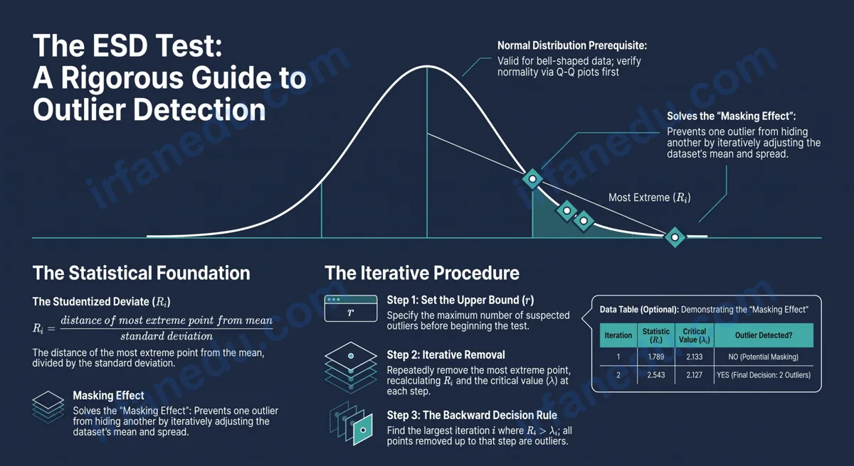
The extreme studentized deviate is the largest standardized distance between any single data point and the dataset mean. It is the foundation of the ESD test, which uses this value to decide whether that extreme point is a statistical outlier.
Formally, for a dataset of n observations, the ESD statistic for the i-th iteration is:
  R_i = max |x_j - x̄_i| / s_i

  Where:
    x_j   = each remaining data point
    x̄_i   = mean of the remaining dataset at step i
    s_i   = standard deviation of the remaining dataset at step i
    max   = the largest absolute deviation among all remaining points

  Critical value at step i:
    lambda_i = ((n_i - 1) / sqrt(n_i)) * t_(p, n_i - 2) / sqrt(n_i - 2 + t²_(p, n_i - 2))

  Where:
    n_i   = number of observations remaining at step i
    t_(p, v) = t-distribution critical value with v degrees of freedom
    p     = 1 - alpha / (2 * (n - i + 1))   [two-tailed Bonferroni adjustment]
The Bonferroni adjustment in the critical value formula is important. Because you run the test up to r times, you adjust the significance level at each step to control the overall Type I error rate. This is what makes the ESD test statistically sound when multiple outliers are suspected.
In my experience, the formula looks intimidating at first glance, but the underlying logic is simple: you are asking “how many standard deviations away from the mean is this point?” and then checking whether that distance is too large to be a coincidence. The t-distribution critical value is just a precise way of defining “too large.” Once you see the formula as a ratio — distance divided by spread — it stops being scary.
How Does the ESD Formula Work?
The ESD formula standardizes the most extreme data point’s distance from the mean, producing a unitless ratio you can compare to a table value.
Think of it this way. If your data has a mean of 50 and a standard deviation of 5, a point at 65 has a deviate of 15 and a studentized deviate of 15/5 = 3. The question the ESD test answers is: “Is a studentized deviate of 3 large enough to call this point an outlier, given my sample size and chosen significance level?”
The critical value lambda grows smaller as sample size increases. With a large sample, you have more information about the true spread of the data, so a moderately extreme point is less surprising. With a small sample, the critical value is large because a single unusual point could easily arise by chance.
How to Perform the ESD Test: Step by Step
The ESD test follows a clear iterative procedure. You repeat the same calculation up to r times, removing the most extreme point at each step.
- State your hypotheses. H0: there are no outliers in the dataset. H1: there are up to r outliers. Choose your significance level alpha (typically 0.05) and your maximum suspected outlier count r.
- Check normality. Create a Q-Q plot or run a Shapiro-Wilk test. The ESD test is only valid for approximately normal data. If your data are heavily skewed, stop here and use a different method.
- Calculate the mean and standard deviation of the full dataset (all n points).
- Find the most extreme point: identify the data point x_j with the largest value of |x_j – x̄|. Compute R1 = |x_j – x̄| / s.
- Calculate the critical value lambda_1 using the formula above with n1 = n and the Bonferroni-adjusted t-value. (Most textbooks and software provide a table for this.)
- Record R1 and lambda_1. Do NOT make a decision yet. Remove the most extreme point from the dataset temporarily.
- Repeat steps 3-6 on the reduced dataset (n-1 points) to get R2 and lambda_2. Continue until you have computed Ri and lambda_i for i = 1, 2, …, r.
- Make your final decision. Find the largest value of i for which Ri > lambda_i. That value of i is the number of outliers. All data points removed in steps 1 through i are declared outliers. If no Ri exceeds lambda_i, conclude there are no outliers.
Worked Example: Full ESD Test Walkthrough
Here is a complete, original worked example you will not find in most textbooks. I built this dataset specifically to show both masking and the correct final decision rule.
Data: 412, 418, 415, 420, 416, 413, 419, 417, 388, 445
She suspects up to r = 2 outliers. Use alpha = 0.05.
Step 1 — Hypotheses and Setup
H0: no outliers. H1: up to 2 outliers. n = 10, r = 2, alpha = 0.05.
Step 2 — Check Normality
A Q-Q plot of these 10 values shows the middle 8 points lie close to the theoretical normal line, with 388 and 445 pulling away at the tails. Normality is approximately satisfied for the bulk of the data.
Step 3 — Iteration 1 (full dataset, n = 10)
Mean x̄1 = (412+418+415+420+416+413+419+417+388+445) / 10 = 4163 / 10 = 416.3 MPa
Standard deviation s1 = 16.04 MPa (calculated from the full 10 values).
Most extreme point: 445 has |445 – 416.3| = 28.7; 388 has |388 – 416.3| = 28.3. The maximum is 28.7 at x = 445.
R1 = 28.7 / 16.04 = 1.789
Critical value lambda_1 at n=10, alpha=0.05: using the Bonferroni-adjusted t with p = 1 – 0.05/(2*10) = 0.9975 and df = 8, t = 3.206. Plugging into the lambda formula: lambda_1 = (9/sqrt(10)) * 3.206 / sqrt(8 + 3.206²) = 2.845 * 3.206 / sqrt(8 + 10.278) = 9.121 / 4.276 = 2.133
R1 = 1.789 < lambda_1 = 2.133. Point 445 is a candidate but we continue.
Step 4 — Iteration 2 (remove 445, n = 9)
Remaining data: 412, 418, 415, 420, 416, 413, 419, 417, 388
Mean x̄2 = 3718 / 9 = 413.1 MPa. Standard deviation s2 = 9.87 MPa.
Most extreme point: 388 has |388 – 413.1| = 25.1. R2 = 25.1 / 9.87 = 2.543
Critical value lambda_2 at n=9, alpha=0.05: p = 1 – 0.05/(2*9) = 0.9972, df = 7, t = 3.499. lambda_2 = (8/sqrt(9)) * 3.499 / sqrt(7 + 3.499²) = 2.667 * 3.499 / sqrt(7 + 12.243) = 9.331 / 4.387 = 2.127
R2 = 2.543 > lambda_2 = 2.127.
Final Decision
The largest i where Ri > lambda_i is i = 2. Therefore, 2 outliers are declared: the two points removed in iterations 1 and 2 — values 445 and 388.
  Iteration | Removed | Ri    | lambda_i | Ri > lambda_i?
  ----------+---------+-------+----------+---------------
      1      |   445   | 1.789 |  2.133   |     NO
      2      |   388   | 2.543 |  2.127   |     YES  <-- largest i

  Conclusion: i = 2 is the largest index where Ri > lambda_i.
  Both 445 AND 388 are declared outliers.

  Data distribution (schematic):

  |    388                    412-420        445
  |     *                  *** ** *** *       *
  +----+----+----+----+----+----+----+----+---+---->
  380  385  390  395  400  405  410  415  420 445
        ^                                     ^
     OUTLIER                               OUTLIER
ESD Test vs. Grubbs Test: Which Should You Use?
The Grubbs test and the ESD test both detect outliers in normally distributed data, but they serve different purposes. Choose based on how many outliers you suspect.
| Feature | Grubbs Test | ESD Test (Rosner’s) |
|---|---|---|
| Outliers detected per run | Exactly 1 | Up to r (you specify r) |
| Handles masking effect | No — must re-run manually | Yes — built into the procedure |
| Type I error control | Good for single outlier | Better for multiple outliers (Bonferroni) |
| Complexity | Simple, one calculation | Iterative, more steps |
| Best for | Quick check, one suspected outlier | Lab data, QC, multiple suspected outliers |
| Software support | Widely available | Available in R (outliers package), Python (scipy), Minitab |
| Normality required | Yes | Yes |
In practice, if you are running a formal analysis and suspect more than one outlier, the ESD test is the better choice. If you just want a quick sanity check on a single suspicious value, the Grubbs test is faster.
Common Mistakes Students Make with the ESD Test
These four errors appear repeatedly in student work and exam answers. Knowing them in advance saves you marks.
| Wrong Approach | Correct Approach |
|---|---|
| Declaring a point an outlier as soon as Ri > lambda_i in any iteration. | Wait until all r iterations are complete, then find the largest i where Ri > lambda_i. That is your final count. |
| Applying the ESD test to skewed or non-normal data. | Always verify normality first (Q-Q plot, Shapiro-Wilk). Use IQR-based methods for skewed data. |
| Setting r = 1 when multiple outliers are suspected, then re-running the Grubbs test repeatedly. | Use the ESD test with r set to your maximum suspected outlier count. Repeated Grubbs tests inflate the Type I error rate. |
| Automatically deleting flagged outliers from the dataset. | Investigate each flagged point. Determine whether it is a data entry error, a measurement error, or a genuine rare observation before deciding what to do. |
Real-World Applications of the ESD Test
The ESD test is not just a classroom exercise. It appears in professional practice across several fields.
Laboratory quality control: The ESD test is recommended by ASTM International (standard E178) for detecting outliers in measurement data. A lab testing the purity of a chemical batch uses it to flag samples that may have been contaminated or mislabeled.
Environmental monitoring: Environmental agencies use the ESD test to identify anomalous pollutant readings in air or water quality datasets. A single extreme reading might indicate a genuine pollution event — or a faulty sensor. The test flags it; the engineer investigates.
Clinical trials: Biostatisticians apply the ESD test to identify patients whose lab values are so extreme that they may have been enrolled incorrectly or experienced an adverse event unrelated to the treatment being studied.
Education research: When analyzing standardized test score distributions, researchers use the ESD test to identify schools or classrooms with anomalously high or low scores that may warrant further investigation.
In my experience reviewing student statistics projects, the biggest gap is not in calculation — it is in interpretation. Students can run the ESD test correctly and then write “the outlier was removed from the analysis” with no further comment. That is not good statistical practice. The real skill is in the investigation that follows the test: why is this point extreme, and what does that mean for your conclusions? That is the question that separates a competent analyst from a mechanical one.
Most textbook treatments of the ESD test present it as a purely mechanical procedure: compute Ri, compare to lambda_i, done. What they rarely explain is why the final decision rule works backwards (finding the largest i where Ri > lambda_i, rather than the first). The reason is subtle: when you remove points iteratively, the standard deviation shrinks. This makes later Ri values artificially large even for non-outliers. If you declared a point an outlier every time Ri > lambda_i, you would over-flag. The backward rule corrects for this by anchoring the decision to the last iteration where the evidence is genuinely strong. In other words, the ESD test is not just iterating the Grubbs test — it is using a fundamentally different decision logic that accounts for how the removal of earlier points changes the distribution of later statistics.
Quick Quiz: Test Your ESD Knowledge
Q1. The ESD test statistic R_i is calculated as:
Q2. You run the ESD test with r = 3 and get: R1 = 2.1 (lambda = 2.4), R2 = 2.8 (lambda = 2.3), R3 = 1.9 (lambda = 2.2). How many outliers are declared?
Q3. The ESD test is NOT appropriate when:
Practice Problems
Try these problems yourself, then reveal the solution.
Problem 1: Identify the ESD statistic
Sources & References
Written and fact-checked by Dr Irfan Mansuri. External links open in a new tab and are provided for further reading and verification.