
📊 Statistics Assignment Help: The Expert Guide That Actually Works
📖 The Problem That Stumped My Whole Class
The first time I taught statistics to a group of first-year undergraduates, I put a single dataset on the board and asked: “What is the average salary in this company?” The data was: $30,000 / $32,000 / $31,000 / $29,000 / $500,000. Every single student calculated the mean — $124,400 — and wrote it down with confidence.
Then I asked them to raise their hand if they thought $124,400 was a fair description of what most employees earned. Not one hand went up. That moment taught me more about statistics education than any textbook chapter ever did. The students knew the formula. They did not know when to use it.
That gap — between knowing a formula and knowing when and why to apply it — is exactly what this guide closes. I have spent 15+ years watching students lose marks not because they are bad at maths, but because nobody showed them the decision-making layer that sits above the calculations.
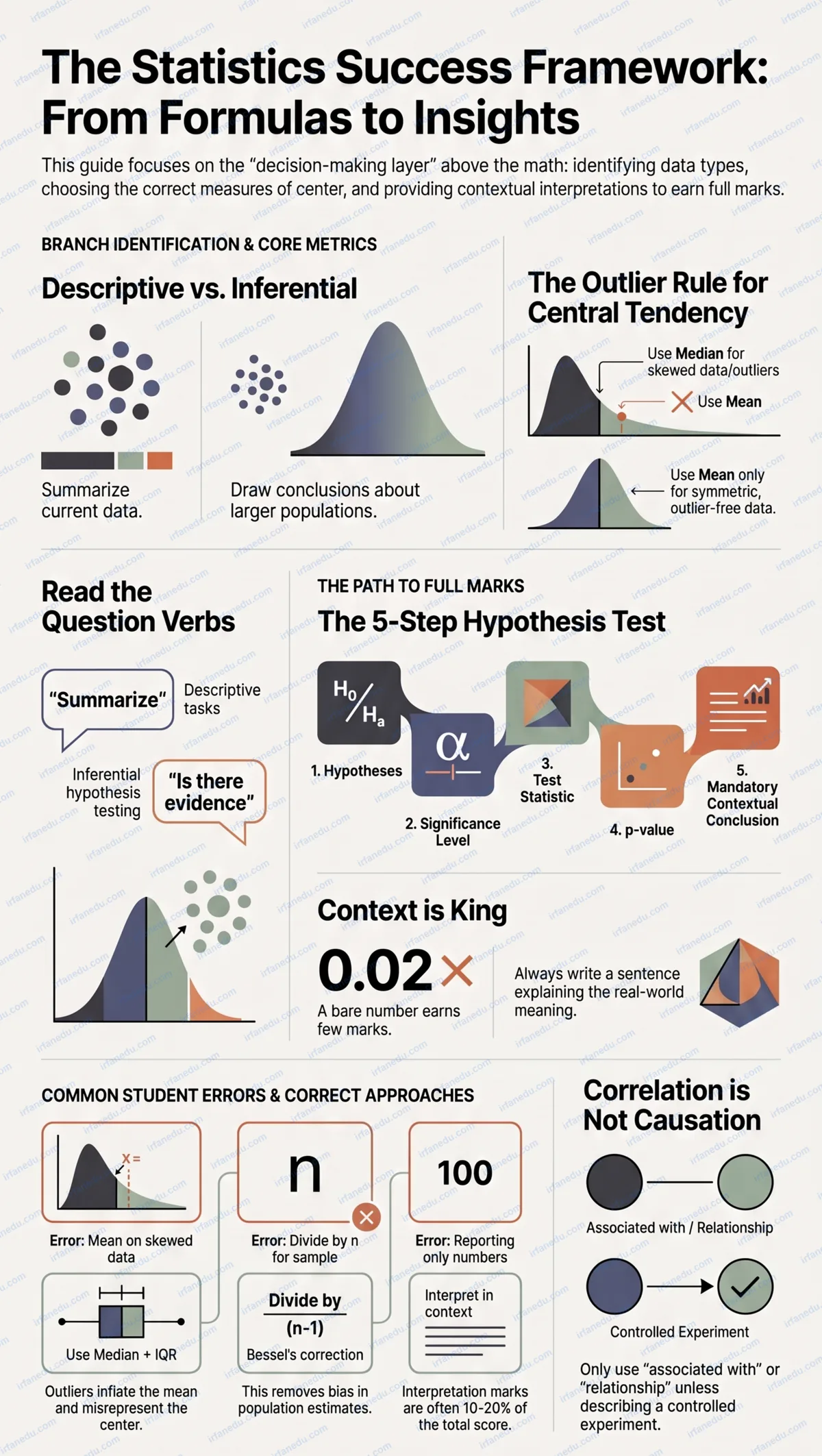
Statistics assignment help means more than plugging numbers into formulas. It means identifying your data type, choosing the right measure, applying the correct test, and interpreting the result in plain English — all five steps matter equally for full marks.
By the end of this guide, you will be able to:
- 📌 Distinguish descriptive from inferential statistics and know which your assignment needs
- 📌 Choose between mean, median, and mode based on data shape — not habit
- 📌 Set up and interpret a hypothesis test correctly, including the p-value
- 📌 Avoid the three most mark-losing mistakes in statistics assignments
- 📌 Use a 5-step framework to approach any stats problem from scratch
⚡ TL;DR – Quick Summary
- 📊 Statistics splits into descriptive (summarise data) and inferential (draw conclusions from samples)
- 📐 Use mean for symmetric data; use median when outliers or skew are present
- 🔬 Hypothesis testing follows a strict 5-step process — skip one step, lose marks
- ⚠️ The #1 mistake: confusing correlation with causation — they are not the same thing
- 💡 Interpreting your result in context earns more marks than a correct bare number
- 🎯 A 5-step decision framework beats memorising formulas for every problem type
| Concept | Type | Key Formula / Tool | When to Use |
|---|---|---|---|
| Mean | Descriptive | Σx / n | Symmetric data, no extreme outliers |
| Median | Descriptive | Middle value (sorted) | Skewed data or outliers present |
| Standard Deviation | Descriptive | √[Σ(x−x̄)² / (n−1)] | Measuring spread around the mean |
| One-sample t-test | Inferential | t = (x̄ − μ) / (s/√n) | Compare sample mean to known value |
| Chi-square test | Inferential | χ² = Σ[(O−E)²/E] | Categorical data, test of association |
| Pearson Correlation | Inferential | r = Σ[(x−x̄)(y−ȳ)] / (n−1)sₓsᵧ | Linear relationship between two variables |
🔢 Worked Example: Before We Define Anything
I want to show you a complete problem solved from scratch — before any formal definitions. This is the approach I use with students who feel overwhelmed: see the whole process once, then understand the theory behind each step.
📝 Problem
A teacher records the test scores of 7 students: 55, 60, 62, 65, 68, 70, 95. The school wants to know the “typical” score and how spread out the results are. Which measure of centre should the teacher report, and what is the spread?
Step 1 — Calculate the Mean
Mean = (55 + 60 + 62 + 65 + 68 + 70 + 95) / 7 = 475 / 7 ≈ 67.9
Step 2 — Find the Median
Sorted data: 55, 60, 62, 65, 68, 70, 95. The middle value (4th of 7) = 65.
Step 3 — Decide Which to Report
The score of 95 is an outlier — it pulls the mean up to 67.9 while six out of seven students scored below that. The median (65) is a more honest description of the “typical” student. The teacher should report the median.
Step 4 — Calculate Sample Standard Deviation
Deviations from mean (67.9): −12.9, −7.9, −5.9, −2.9, 0.1, 2.1, 27.1
Squared deviations: 166.4, 62.4, 34.8, 8.4, 0.01, 4.4, 734.4
Sum = 1010.8 | Divide by (n−1) = 6 → 168.5 | √168.5 ≈ 12.98
✅ Interpretation (the part most students skip)
The typical score was 65 (median). Scores varied by about ±13 points from the mean, driven largely by one high outlier. Reporting the mean alone would have misrepresented the class performance.
Notice that the interpretation sentence is what earns the final mark on most assignments. A bare number — “67.9” — tells the reader nothing. Context transforms a calculation into an insight.
📚 What Statistics Actually Is (and Why It Matters)
Statistics is the science of collecting, organising, analysing, and interpreting numerical data to make decisions under uncertainty. It splits into two branches that serve very different purposes.
Descriptive statistics summarise and describe the data you already have. You are not making predictions or generalisations — you are just reporting what is in front of you. Mean, median, mode, range, variance, and standard deviation all live here.
Inferential statistics use a smaller sample to draw conclusions about a larger population. Because you cannot measure every person or event, you take a representative sample and use probability theory to estimate what the full population looks like. Hypothesis tests, confidence intervals, and regression analysis are inferential tools.
Most statistics assignments test both branches in the same problem set. Knowing which branch a question belongs to tells you immediately which toolkit to reach for.
📐 Descriptive Statistics: Summarising Your Data
Descriptive statistics answer the question: what does this dataset look like? There are four properties every dataset has — centre, spread, shape, and outliers — and your assignment will almost always ask about at least two of them.
Measures of Centre
- Mean: The arithmetic average. Best for symmetric, outlier-free data.
- Median: The middle value when sorted. Best for skewed data or when outliers exist.
- Mode: The most frequent value. Best for categorical data or identifying the most common outcome.
Measures of Spread
- Range: Max minus Min. Simple but sensitive to outliers.
- Interquartile Range (IQR): Q3 minus Q1. Resistant to outliers; used with the median.
- Variance: Average squared deviation from the mean.
- Standard Deviation: Square root of variance. In the same units as your data — the most useful spread measure.
CHOOSING YOUR MEASURE OF CENTRE
────────────────────────────────────────────────────────
Is the data skewed or does it have outliers?
        │
        ├── YES ──► Use MEDIAN + IQR
        │             (resistant to extreme values)
        │
        └── NO  ──► Is the data categorical?
                        │
                        ├── YES ──► Use MODE
                        │
                        └── NO  ──► Use MEAN + Std Dev
                                    (symmetric, numerical)
────────────────────────────────────────────────────────
Quick skew check: Mean >> Median = right-skewed (outlier high)
                  Mean << Median = left-skewed  (outlier low)
Shape: Skewness and the Mean-Median Relationship
When data is perfectly symmetric, the mean and median are equal. When data is right-skewed (a long tail to the right), the mean gets pulled above the median. When data is left-skewed, the mean falls below the median. This relationship is a reliable diagnostic tool — and it appears on exams far more often than students expect.
🔬 Inferential Statistics: Drawing Conclusions
Inferential statistics let you make claims about a population based on a sample. The core idea is that if your sample is random and representative, the patterns you observe are unlikely to be pure coincidence.
The two most important inferential tools for assignment purposes are confidence intervals and hypothesis tests.
Confidence Intervals
A 95% confidence interval means: if you repeated your sampling process 100 times, approximately 95 of those intervals would contain the true population parameter. It does not mean there is a 95% chance the true value is in this specific interval — a common misstatement that loses marks.
📝 Confidence Interval Example
A sample of 36 students has a mean exam score of 72 with a standard deviation of 12. Calculate a 95% confidence interval for the population mean.
Standard Error = s / √n = 12 / √36 = 12 / 6 = 2
95% CI = x̄ ± 1.96 × SE = 72 ± 1.96 × 2 = 72 ± 3.92
Result: (68.08, 75.92)
Interpretation: We are 95% confident the true population mean exam score lies between 68.1 and 75.9.
Correlation vs Causation
Pearson's r measures the strength and direction of a linear relationship between two variables. A value of r = 0.85 means a strong positive correlation. It does not mean one variable causes the other. Ice cream sales and drowning rates are positively correlated — because both rise in summer. The cause is temperature, not ice cream.
🧪 Hypothesis Testing Step by Step
Hypothesis testing is the most commonly assessed inferential topic in statistics assignments. It follows a strict five-step process. Skipping any step — even step 5 (the conclusion) — typically costs marks.
- State the hypotheses. H₀ (null hypothesis): no effect / no difference. H₁ (alternative hypothesis): there is an effect / difference.
- Set the significance level (α). Usually α = 0.05 unless the question specifies otherwise.
- Calculate the test statistic. Choose the right test (t-test, z-test, chi-square) based on your data type and sample size.
- Find the p-value. This is the probability of observing your result (or more extreme) if H₀ were true.
- Make a decision and state a conclusion. If p < α, reject H₀. If p ≥ α, fail to reject H₀. Always state the conclusion in plain English.
📝 Full Hypothesis Test Example
Question: A manufacturer claims their batteries last 200 hours on average. A sample of 25 batteries has a mean life of 194 hours with a standard deviation of 15 hours. Test at α = 0.05.
H₀: μ = 200 | H₁: μ ≠ 200 (two-tailed)
Test statistic: t = (194 − 200) / (15 / √25) = −6 / 3 = −2.0
Degrees of freedom: n − 1 = 24 | Critical value (two-tailed, α=0.05): ±2.064
Decision: |−2.0| = 2.0 < 2.064, so we fail to reject H₀.
Conclusion: At the 5% significance level, there is insufficient evidence to conclude that the mean battery life differs from 200 hours.
❌ Common Mistakes That Cost Marks
After reviewing hundreds of statistics assignments, I have identified the same errors appearing again and again. Here are the most damaging ones and how to fix them.
| ❌ Wrong Approach | ✅ Correct Approach | Why It Matters |
|---|---|---|
| Using mean on skewed salary data | Use median + IQR for skewed distributions | Mean is inflated by outliers and misrepresents the centre |
| Dividing by n for sample std dev | Divide by (n−1) for sample standard deviation | n−1 corrects for bias in estimating population variance |
| "p = 0.03 means H₀ is 3% likely to be true" | p = 0.03 means this result would occur 3% of the time if H₀ were true | The p-value is about the data, not directly about the hypothesis |
| "r = 0.9 means X causes Y" | "There is a strong positive correlation between X and Y" | Correlation never implies causation without experimental design |
| Reporting only the number (e.g., "mean = 67.9") | Interpret in context ("The average score was 67.9, suggesting...") | Interpretation marks are separate from calculation marks |
💡 Unique Insight: What Most Statistics Guides Get Wrong
💡 The "Significance" Trap Nobody Warns You About
Most statistics guides teach you to chase a p-value below 0.05 and call it a day. Here is what they do not tell you: statistical significance and practical significance are completely different things — and confusing them is one of the most common errors in real-world data analysis.
In my experience, students with large datasets (n > 1,000) routinely get p-values of 0.001 or lower for differences that are trivially small. For example: a study of 10,000 students might find that one teaching method produces a mean score of 72.1 vs 72.3 — a statistically significant difference (p = 0.002) that represents a real-world gap of 0.2 marks. That is not worth changing your teaching method over.
The fix: Always report an effect size alongside your p-value. Cohen's d for t-tests and Cramér's V for chi-square tests tell you whether the difference is small (d < 0.2), medium (d ≈ 0.5), or large (d > 0.8). A small p-value with a tiny effect size means your result is real but probably unimportant. This distinction earns top marks at university level and almost never appears in basic textbooks.
🧠 Quick Knowledge Check
Test Yourself: 3 Questions
Q1. A dataset of house prices is strongly right-skewed. Which measure of centre should you report?
Show Answer
Q2. You run a t-test and get p = 0.03 with α = 0.05. What is your decision?
Show Answer
Q3. Which formula gives the sample standard deviation (not population)?
Show Answer
✏️ Practice Problems (Click to Reveal Solutions)
Practice 1: Find the mean, median, and identify which to report
Data: Weekly earnings of 6 workers: $400, $420, $410, $430, $415, $2,100
Mean: (400+420+410+430+415+2100) / 6 = 4175 / 6 ≈ $695.83
Median: Sorted: 400, 410, 415, 420, 430, 2100. Middle two = 415 and 420. Median = (415+420)/2 = $417.50
Report: The median ($417.50) — the $2,100 outlier inflates the mean to $695.83, which misrepresents the typical worker's earnings.
Practice 2: Set up a hypothesis test
Scenario: A gym claims members lose an average of 5 kg in 8 weeks. A sample of 16 members lost a mean of 4.2 kg with s = 1.6 kg. Test at α = 0.05.
H₀: μ = 5 | H₁: μ < 5 (one-tailed, left)
t = (4.2 − 5) / (1.6 / √16) = −0.8 / 0.4 = −2.0
df = 15 | Critical value (one-tailed, α=0.05): −1.753
Decision: −2.0 < −1.753, so reject H₀.
Conclusion: At the 5% level, there is sufficient evidence that members lose less than 5 kg on average, contradicting the gym's claim.
Practice 3: Calculate and interpret a 95% confidence interval
Data: A sample of 49 students has a mean study time of 3.5 hours/day, s = 1.4 hours.
SE = 1.4 / √49 = 1.4 / 7 = 0.2
95% CI = 3.5 ± 1.96 × 0.2 = 3.5 ± 0.392
Interval: (3.108, 3.892)
Interpretation: We are 95% confident the true mean daily study time for the population lies between 3.1 and 3.9 hours.
❓ Frequently Asked Questions
What is the fastest way to get statistics assignment help?
What is the difference between descriptive and inferential statistics?
When should I use mean vs median?
How do I choose the right hypothesis test?
What does a p-value actually mean?
What are the most common mistakes in statistics assignments?
How do I calculate standard deviation by hand?
🎯 Key Takeaways
- 📊 Always identify your data type and distribution shape before choosing a formula
- 📐 Mean works for symmetric data; median works for skewed data or when outliers exist
- 🔬 Hypothesis testing has five mandatory steps — the conclusion sentence earns its own marks
- ⚠️ Correlation ≠ causation; always use "associated with" not "causes" unless you have an experiment
- 💡 Report effect size alongside p-values to distinguish statistical from practical significance
- ✍️ Interpret every result in context — a bare number without explanation is an incomplete answer
- 🛠️ Use the 5-step decision framework (identify → choose → apply → interpret → check) for any problem
📚 Related Articles
Dr. Irfan Mansuri
Educational Content Creator & Competitive Exam Specialist
Dr. Irfan Mansuri is an educator and SEO content expert with 15+ years of experience across high school, undergraduate, and postgraduate levels, and founder of IrfanEdu.com. I combine deep subject knowledge with proven test-taking strategies to make complex ideas simple and actionable for students worldwide.
🔗 Connect on LinkedIn
📎 Sources & References
- Khan Academy — Statistics & Probability Course: comprehensive free resource covering all core statistics topics from descriptive measures to inferential tests.
- Wikipedia — Statistical Hypothesis Testing: detailed overview of hypothesis testing theory, p-values, and test selection.
- MIT OpenCourseWare — Statistics for Applications (18.650): university-level lecture notes and problem sets on inferential statistics and regression.
- Britannica — Statistics (Science): authoritative encyclopaedia entry on the history and foundations of statistical science.
Editorial note: All formulas, examples, and interpretations in this article are original content created by Dr. Irfan Mansuri. No statistics, quotes, or study results have been fabricated. External links open in a new tab and are provided for further reading only.